9. A Template: Solow-Swan’s Growth Mechanism#
The Solow [29] and Swan [31] model is our starting point.
We will use it for postulating hypotheses about and analyzing the causes and consequences of economic growth. The model also serves as a backbone for much of modern macroeconomic models.
We will use this structure to also to perform thought experiments, or comparative statics, to understand what factors might contribute to greater levels of income per capita and what might account for faster economic growth.
As a starting or reference point, the Solow-Swan model will also expose what is missing from economists’ understanding of basic causes of economic growth. In short, the model paves the way for several generations of improvements to our basic theory and empirical work to test these theories.
9.1. Environment#
Let’s begin with the simplest version of this model without growth in population or technology.
Primitives. Solow and Swan share a Keynesian modelling taste when it comes to behavioral abstraction. Specifically, they avoid discussing the basic underpinnings of how agents come to act according to particular behavioral patterns or rules. That is, behavior in the model is hard wired.
The only aspect that is crucially fundamental to the Solow-Swan model is a description of the production set:
A goods-production function that transforms technology, labor and capital into a final good; and
a capital-accumulation technology that transforms existing (undepreciated) capital and new investments into more capital.
Actors. The model has the following economic agents:
an infinite set of identical households; and
an infinite set of identical and perfectly competitive firms.
Trading environment. They interact as price takers in the following Walrasian markets:
A market for a single good;
a labor market; and
a capital market.
Economic equilibrium concept. General equilibrium at each point in time arises when demand equals supply of the commodity traded in each market.
9.1.1. Production#
The main ingredients driving economic growth in the Solow-Swan model are
Exogenous technological or technical progress, \(A(t)\);
the neoclassical idea of physical capital, \(K(t)\), and labor, \(L(t)\), as inputs into a constant-returns-to-scale, goods-production function \(F\);
a capital-production technology that transforms new investments and existing capital into more capital for the future.
The goods-production function is given by
We make the following assumption regarding returns to scale of production:
Property 9.1
The production function \(F\) is linearly homogeneous or homogeneous of degree \(m=1\) in capital, \(K(t)\), and labor, \(L(t)\).
What does linear homogeneity of a function in its arguments mean?
Definition 9.1
Let \(z \in \mathbb{R}^{N}\) for some \(N \geq 1\) denote a list of many variables. The function \(g(x, y, z)\) is homogeneous of degree \(m\) in the two variables, \(x \in \mathbb{R}\) and \(y \in \mathbb{R}\), if and only if
for all \(\lambda \in \mathbb{R}_{+}\) and \(z \in \mathbb{R}^{N}\).
Example 9.1 (Constant returns to scale)
Suppose \(m=1\) and \(\lambda=2\). In this case, what Definition 9.1 tells us is that if we double the inputs \((x,y)\) while keeping all else fixed, the function \(g(\cdot, z)\) returns a doubling of the output.
Exercise 9.1
Show that if \(F\) is linearly homogeneous in \(K\) and \(L\), then it is (weakly) concave in \(K\) and \(L\).
We will also impose more structure on \(F\):
Property 9.2
\(F\) is
twice continuously differentiable in \(K\) and \(L\);
increasing in its endogenous inputs: \(\partial F(A,K,L)/\partial K > 0\) and \(\partial F(A,K,L)/\partial L > 0\);
increasing in \(A\), and \(A\) is positive-valued; and
strictly concave in its endogenous inputs (diminishing returns to capital and labor): \(\partial^{2} F(A,K,L)/\partial K^{2} < 0\) and \(\partial^{2} F(A,K,L)/\partial L^{2} < 0\).
The degree of diminishing returns to capital will be crucial to many results of the Solow-Swan model.
If \(F\) is continuously differentiable and linearly homogeneous in the factors of production \(K\) and \(L\), then total output can be accounted for by the sum of all the marginal product of each input times the quantity of each input. This is a consequence of the following more general observation:
Theorem 9.1 (Euler’s Theorem)
Suppose that \(g : \mathbb{R}^{N+2} \rightarrow \mathbb{R}\) is continuously differentiable in \(x\in\mathbb{R}\) and \(y\in\mathbb{R}\), with partial derivatives denoted by \(g_{x}\) and \(g_{y}\) and is homogeneous of degree \(m\geq1\) in \(x\) and \(y\).
Then
for all \(x\in\mathbb{R}\), \(y\in\mathbb{R}\) and \(z\in\mathbb{R}^{N}\).
Furthermore, \(g_{x} (x, y, z)\) and \(g_{y} (x, y, z)\), respectively, are homogeneous of degree \(m-1\) in \(x\) and \(y\).
Exercise 9.2
Prove Euler’s Theorem.
Use it to verify our statement above for the example where \(F(A,K,L)=K^{\alpha}(AL)^{1-\alpha}\) and \(0<\alpha<1\).
What does this mean for firms’ profits? Does ownership structure matter in this model economy?
We will assume that
Property 9.3
\(F\) satisfies the Inada conditions:
\(\lim_{K \rightarrow 0} F_{K}(A,K,L) = \infty\) and \(\lim_{K \rightarrow \infty} F_{K}(A,K,L) = 0\) for all \(L>0\) and all \(A\).
\(\lim_{L \rightarrow 0} F_{L}(A,K,L) = \infty\) and \(\lim_{L \rightarrow \infty} F_{L}(A,K,L) = 0\) for all \(K>0\) and all \(A\).
These conditions help ensure that equilibria are away from corner solutions.
9.1.2. Capital accumulation#
At each moment, households own capital stock \(\bar{K}(t)\) which gets rented out to firms.
Capital stock wears out—due to its use in production—at rate \(\delta \in (0,1)\).
Capital-production transforms new investment, \(I(t)\), net of depreciated capital, to determine the rate of change in \(\bar{K}(t)\):
9.1.3. Economic actors and actions#
Let’s begin with the actors: households and firms.
Every household supplies one unit of labor to the labor market.
The labor force is thus \(\bar{L}(t)\). This is also the population size.
At each \(t\), households consumes a fraction \((1-s) \in (0,1)\) out of total income,
at each instance \(t\).
What is not consumed is saved:
Saving goes into the investment good \(I(t)\). This adds to capital accumulation (9.2).
Firms hire workers \(L(t)\) and capital \(K(t)\) to produce output.
This transformation uses a constant returns-to-scale production function (9.1).
Firms take the rental price of labor (\(w\)) and capital (\(R\)), measured in units of \(Y\), as given.
The demand for labor and capital are
and
respectively.
Exercise 9.3
Normalize the price level of the final good to 1.
The representative firm maximizes its profit which is the difference between the revenue from selling its final good \(Y(t)\) and the rental costs of labor capital services.
Write down the profit function. Show that the optimal price-taking behavior of the firm is given by the factor demand schedules (9.5) and (9.6).
9.1.4. Market clearing and competitive equilibrium#
Markets are Walrasian. These markets are for the exchange of labor and capital services, and for the final good.
Demand and supply of factors of production must equal at each moment in time:
and,
Exercise 9.4
Sketch accurate depictions of the demand and supply curves for these factors of production. (For example, label \(K(t)\) on the horizontal axis and \(R(t)\) on the vertical axis for the capital market diagram.) Show the allocation-price pair that satisfy (9.7) and (9.8) in each respective diagram.
Definition 9.2 (Competitive equilibrium)
Given an exogenous \(t \mapsto A(t)\), a competitive equilibrium is an allocation and pricing trajectory, respectively, \(t \mapsto (K, L)(t)\) and \(t \mapsto (w, R)(t)\) such that
Exercise 9.5
Show that it suffices to describe the (dynamic) competitive equilibrium by the following equations determining the solution for \(t \mapsto (K, L)(t)\):
and Equation (9.8).
9.2. Setting with population growth#
Let’s now redo the same setting as before, but now, we allow for the population to grow.
Exercise 9.6 (Solow-Swan with population growth)
Assume that labor force (and population) grows at exponential rate \(n\):
Also, assume that productivity is constant, \(A(t)=A>0\), for all \(t\).
Given that \(F\) has constant returns to scale, show that it suffices to describe the (dynamic) competitive equilibrium by the following equations determining the solution for \(t \mapsto k(t)\):
where \(k(t):=K(t)/L(t)\) and \(f(k(t), A) = F(k(t), 1, A)\).
It turns out that the final-good market also must clear. We get this “for free”.
Exercise 9.7
Derive the expression of the final-good market clearing condition from the equilibrium definition above.
9.3. Steady-state equilibrium and comparative statics#
What is the economy’s equilibrium like if the state of the economy remains stable or unchanged over time?
Consider the version of Solow-Swan with population growth in Exercise 9.6.
Here, the state variables would be \(K(t)\) and \(L(t)\). However, because population is growing, we need to have a well-defined notion of a steady state. If we work with the “detrended” variable \(k(t) := K(t)/L(t)\), then there is a well-defined steady state:
Exercise 9.8
Show that a steady-state equilibrium for the dynamic equilibrium or ODE in Equation (9.10) is a point \(k^{\star}\) satisfying
Given our assumptions above about \(F\), is the steady state equilibrium unique? Get your intuition straight by drawing the appropriate graphs representing Equation (9.11).
Can you put into words what this steady-state equilibrium condition says? What forces are being balanced here such that the economy is at rest or at a steady state?
Exercise 9.9
Prove that there is a unique nontrivial steady-state equilibrium point, \(k^{\star} > 0\), satisfying Equation (9.11).
Show that \(k^{\star}\) is
increasing in \(A\) and \(s\), and
decreasing in \(n\) and \(\delta\).
What about income and consumption?
Explain your findings in words, using the model’s reasoning.
9.4. Transitional dynamics#
The dynamic equilibrium of Solow-Swan’s economy is quite straightforward:
Proposition 9.1
Assume all the properties stated earlier about \(F\): Property 9.1, Property 9.2 and Property 9.3.
If the initial state of the Solow-Swan economy in Exercise 9.6 is away from the steady state \(k^{\ast}>0\), it will converge monotonically to \(k^{\ast}\).
Exercise 9.10 (Monotone equilibrium dynamics)
Use the equilibrium map described by Equation (9.10). Show that the steady state \(k^{\ast}>0\) of this nonlinear ODE is not only locally, but also globally, asymptotical stable.
Let’s take a look at a numerical example.
Show code cell source
import numpy as np
import matplotlib.pyplot as plt
from scipy import optimize
We need to define the equilibrium map (ODE):
In a numerical example, we’ll need to instantiate or parametrize the function \(f\).
Let’s suppose it is Cobb-Douglas:
Example 9.2
Assume \(A = 1, \alpha=1/3, s = 1/4, n=1/1000, \delta=7/100\), and,
Show code cell source
def f(k, A, α):
    """Cobb-Douglas instance of per-worker
    production function"""
    return (k**α)*(A**(1.0-α))

def saving(k, A, α, s):
    """Momentary savings flow"""
    return s*f(k, A, α)

def claims(k, n, δ):
    """Momentary claims on capital: depreciation,
    population growth"""
    return (n+δ)*k

def g(k, A=1.0, α=0.33, s=0.25, n=0.001, δ=0.07):
    """Competitive equilibrium map or ODE"""
    return saving(k, A, α, s) - claims(k, n, δ)
Let’s also calculate the steady state, which will come in handy as a reference point. A steady state, \(k^{\ast}\), in this example satisfies
Simplifying, we have
or \(k^{\ast} = 0\).
There are two possible steady states. We’ll focus on the non-zero steady-state case.
We can also find this numerically as a root-finding problem involving a continuous and monotone map on the domain \([k_{\min}, k_{\max}]\), where \(0< k_{\min} < k_{\max} < \infty\).
Given the example, you should get:
Show code cell source
k_min = 0.0001 # Set away from 0
k_max = 10000.0 # Set arbitrarily large
kbar = optimize.brentq(g, k_min, k_max)
print("Non-zero steady state equilibrium = ", kbar)
Non-zero steady state equilibrium = 6.5454992291302565
Draw the equilibrium map on the \((k,\dot{k})\) plane:
Show code cell source
# Specify sample grid points in state space
k_min = 0.0
k_max = kbar*1.88
Ngrid = 238
X = np.linspace(k_min, k_max, Ngrid)

bump = 1.0
X_zoom = np.linspace(k_min+bump, k_max, Ngrid)
Show code cell source
plt.figure()
plt.plot(X, g(X), label=r"$g$")
plt.plot(X, 0.0*X, label=r"$\dot{k}(t)=0$")
plt.plot(kbar, 0.0, 'or')
plt.xlabel(r"$k(t)$")
plt.ylabel(r"$\dot{k}(t)$")
plt.legend();
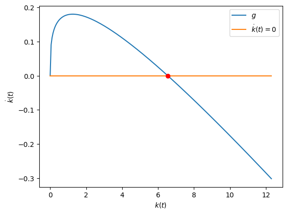
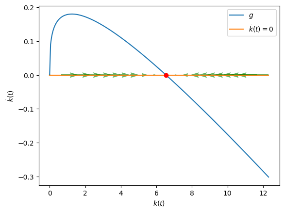
From the shape of this map, and more precisely, using the formula for \(g\), we can calculate the phase line for this model.
This will tell us the dynamic tendencies of the Solow-Swan equilibrium:
Show code cell source
# Coordinates - 1D example, so y = 0
x = np.linspace(X.min(), X.max(), 20)
y = np.zeros(x.shape)

# Directions/gradients - 1D example, so v = 0
# magnitude = length of arrow
# sign = direction
u = g(x)
v = np.zeros(u.shape)
Show code cell source
plt.figure()
plt.plot(X, g(X), label=r"$g$")
# Reference line for zero-growth locus and steady state point
plt.plot(X, 0.0*X, label=r"$\dot{k}(t)=0$")
plt.plot(kbar, 0.0, 'or')
# Vector field (u,v) at each (x,y)
Q = plt.quiver(x, y, u, v,
               color="green",
               alpha=0.6)
plt.xlabel(r"$k(t)$")
plt.ylabel(r"$\dot{k}(t)$")
plt.legend();
We can also see the same thing in \((k, \dot{k}/k)\) space:
Show code cell source
plt.figure()
plt.plot(X_zoom, g(X_zoom)/X_zoom, label=r"$g$")
# Reference line for zero-growth locus and steady state point
plt.plot(X_zoom, 0.0*X_zoom, label=r"$\dot{k}(t)=0$")
plt.plot(kbar, 0.0, 'or')
# Vector field (u,v) at each (x,y)
Q = plt.quiver(x, y, u, v,
               color="green",
               alpha=0.6)
plt.xlabel(r"$k(t)$")
plt.ylabel(r"$\frac{\dot{k}(t)}{k(t)}$")
plt.legend();
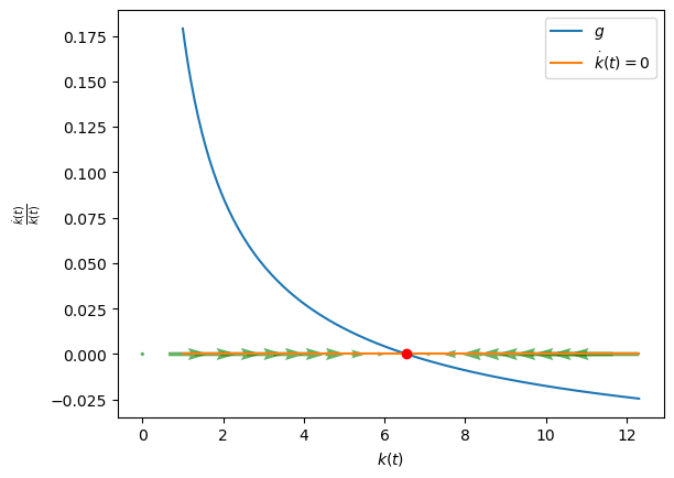
This alternative picture gives us a direct measure of the size and direction of growth of the Solow-Swan equilibrium, when it is evaluated at any possible current state \(k(t)\).
9.5. How to attain perpetual growth?#
From what we just saw, it seems that if the Solow-Swan model has its state \(k(t)\) away from \(k^{\ast}\), it will converge in a monotone way towards \(k^{\ast}\).
What that means is that in the so-called long run, where \(k(t)=k^{\ast}\) for all \(t\), the economy would attain a perpetually constant living standard: It would not grow indefinitely.
How would one hack this model to make it produce long-run or perpetual growth?
9.5.1. A first-step (backwards in time)#
Suppose we relax the restrictions imposed earlier (i.e., Property 9.1, Property 9.2 and Property 9.3).
Exercise 9.11
Let’s reconsider Example 9.2. Now set \(\alpha=1\).
Show that the competitive equilibrium ODE becomes
This is a version of a much earlier growth model, the “AK” model, due to Harrod [10] and Domar [8].
Is there a stable steady state equilibrium? Why or why not?
What is the growth rate of capital and income per person in this model? What is needed for this model to exhibit perpetual growth in \(k\)?
What happens to the ratio of capital income to national income (or the capital share in national income)—i.e., \(R(t)K(t)/Y(t)\)—in this model in as time goes on?
Is this model counterfactual in a particular way?
9.5.2. Exogenous (labor-augmenting) technological progress#
What sort of technological progress?
We shall see that some empirical regularities, first documented by Nicolas Kaldor, restrict the possible ways we can model technological progress.
Kaldor facts
As per capita output and capital increase over time, the
capital-output ratio,
the real interest rate, and
the share of income between capital and labor
remain roughly constant.
Growth economists refer to a path of an economy consistent with these properties as balanced growth path (BGP).
Acemoglu [1] discussed three avenues through which the notion of “technological progress” may augment the production model:
\(A_{H}(t)\) is called Hicks-neutral technological progress.
\(A_{K}(t)\) is called Solow-neutral or capital-augmenting technological progress.
\(A_{L}(t)\) is called Harrod-neutral or labor-augmenting technological progress.
Exercise 9.12
Draw the input \(K\) on the horizontal axis. Place input \(L\) on the vertical axis. (Recall your lessons on production sets and isoquants from intermediate microeconomics?)
Suppose \(F\) is a representation of a strictly convex production set. Depict a few isoquants induced by \(F\).
Show what happens to the isoquants when there is an increase in:
\(A_{H}(t)\) only;
\(A_{K}(t)\) only; and,
\(A_{L}(t)\) only.
As the title of this section suggests, only the Harrod-neutral or labor-augmenting case will be consistent with a BGP.
Why is that?
An intuitive answer comes from inspecting the constant-returns-to-scale production function with labor-augmenting technical progress. Suppose the production function has this form:
If we divide both sides by \(Y(t)\), we have
To exhibit a BGP, capital must be growing just as fast as output, so that the ratio \(K(t)/Y(t)\) is constant, as observed by Kaldor. If labor does not inherit the trend in output, then the ratio \(L(t)/Y(t)\) will not be constant. To ensure balance in Equation (9.12), one would require \(A(t)\) to be growing at a rate that is the gap between the growth rates of output and labor.
Notice how this intuitive argument relies only on the production side of the economy, i.e., on \(F\); and not on descriptions of market-equilibrium behavior?
Let’s summarize this more formally as the steady-state or balance-growth theorem. In words, it says that if a neoclassical growth model exhibits balanced or steady-state growth, then technological progress must be labor augmenting, at least at some point in time consistent with observing balanced-growth.
Proposition 9.2 (Uzawa’s balanced-growth theorem)
Assume a growth model with a constant-returns-to-scale aggregate production function
where \(\tilde{A}\) is technology at time \(t\) and population grows at a constant rate:
Suppose the aggregate resource constraint is
Also, assume that there is an asymptotic path (i.e., for sufficiently large \(t\)) where growth rates of output, capital and consumption become constant, respectively, \(\dot{Y}(t)/Y(t) = g_{Y}\), \(\dot{K}(t)/K(t) = g_{K}\), and \(\dot{C}(t)/C(t) = g_{C}\), and, \(g_{K}+\delta>0\).
Then
\(g_{Y} = g_{K} = g_{C}\); and
asymptotically, the production function can be expressed with a labor-augmenting technology:
where
The proof is given in Acemoglu [1]. This proposition, due to Schlicht [27], is a stronger version of the original Uzawa [32] insight. See Jones and Scrimgeour [13] for further exposition.
Exercise 9.13
Explain verbally the essence of the proof of Proposition 9.2 in Acemoglu [1].
What is remarkable or notable about the result?
Exercise 9.14
Verify Proposition 9.2 for the case of a constant-elasticity-of-substitution (CES) production function. See Example 2.3 in Acemoglu [1].
Exercise 9.15
Show that whether technology is modelled as Hicks-, Harrod- or Solow-neutral is irrelevant for the case where the production function has a Cobb-Douglas form.
Why?
Let’s now work with the production featuring Harrod-neutral technological progress:
Exercise 9.16
Show that the Solow-Swan model with labor-augmenting technological progress has a dynamic equilibrium summarized by the ODE:
where \(k:=K/AL\) denotes the effective capital-labor ratio and \(f(k) \equiv F[K/AL, 1]\).
Per-worker income is:
9.6. Comparative dynamics#
We can show that with Harrod-neutral technical progress, there is a steady-state equilibrium (measured in terms of effective per-worker capital), \(k^{\ast}>0\). At \(k^{\ast}>0\), the economy just balances out the force of saving on capital-stock growth against its countervailing forces. These opposing forces arise from
“capital shallowing” through depreciation (\(\delta\)), and,
“capital narrowing” due to a more efficient (\(g\)) and larger (\(n\)) workforce.
Exercise 9.17
Sketch a phase plot in \((k, \dot{k}/k)\)-space.
Illustrate the dynamics of the model above when \(k(t)\) is away from \(k^{\ast}>0\).
Separately, illlustrate and explain what happens to the steady state and the transitional dynamics if
\(g\) increased;
\(n\) decreased; or
\(\delta\) increased
permanently?
9.7. Takeaways#
Through Solow-Swan, we now have a simple and tractable model of capital accumulation.
It provides us with a launchpad for figuring out what drives permanent growth: Harrod-neutral or labor-augmenting technological change.
However, earlier, we asked why some countries are rich while others are poor; why some grow while others don’t.
The Solow model can help us account for the first question about cross-country differences in income per worker.
But in order to account for why some countries grow while others don’t it requires an exogenous technological growth hack.
Later we will try to unpack this black-box object called technological progress, by asking which factors drive technological progress.
A second deficiency about the Solow-Swan model is that the rate of capital accumulation is determined by the saving rate, the depreciation rate and the rate of population growth—all exogenous objects in the theory.
We should view these “deficiencies” as doors to open questions. Despite these theoretical silences in the model, it is still a useful structure for empiricists to start out in testing a bunch of growth hypotheses in the data. We resume this point in the upcoming topic!