11. Optimal Control Theory#
This is a concise review of the idea and method of optimal control theory. One seeks the best control for taking a dynamical system from one state to another in the presence of constraints on the state and input controls.
What do we mean by “best”? What is a “control”? Read on.
We will survey the main insight of optimal control theory—the Maximum Principle due to Pontryagin, Boltyanskii, Gamkrelidze, and Mischenko [20].
Also known as Pontryagin’s Maximum Principle (PMP), the technique provides a generalization of the classical calculus of variations.
Ramsey [22] was the first to pose and solve the question: What is the path of consumption or investment that attains the greatest lifetime happiness (or least resource-expenditure cost) for an individual (planner), when the state of economic wealth evolves over time depending on the chosen decision path?
We will also see that under convexity restrictions, the PMP is a dual to a sufficient formulation in the form of Bellman’s Principle of Optimality (BPO) [7]. The BPO has a very intuitive and somewhat natural appeal. It requires that whatever the initial state and past actions, the remaining decisions must be selections from an optimal control. This leads one to think about solving an infinitely-large problem by means of “backward induction”—i.e., by solving equivalent small and finite-dimensional problems.
Takeaways
Neccessity. The PMP will say that it is necessary for any optimal control and its induced optimal trajectory of the state to satisfy
a two-point boundary value problem (BVP) known as a Hamiltonian; and
a maximum condition of the control Hamiltonian.
Bang for the math buck! This transforms the original optimal control problem (selections from infinite-dimensional function space), to a point-wise problem summarized by an ODE.
Sufficiency. From a very intuitive marginal-cost-versus-benefit requirement, we can derive a partial differential equation (PDE) in the value of the optimal control problem. This PDE, known as the Hamilton-Jacobi-Bellman (HJB) equation, uniquely determines the optimal value function \(V\) (or “indirect utility” for the economics student). Armed with solution \(V\), this also gives us the necessary conditions for constructing an optimal control solution. Together, we have the BPO.
The PMP necessary conditions are also sufficient (i.e., agree with HJB) under additional convexity restrictions on the objective and constraint functions.
In economies where the fundamental welfare theorems of general equilibrium hold this will imply that decentralized (competitive) equilibrium can be solved as a social planning problem.
In economies—e.g., with externalities, market power, contractual frictions—where these fail the solution to PMP need not be socially optimal and thus not coincide with the HJB formulation.
11.1. Motivation and defining our turf#
Controllable dynamical system. Consider a dynamical system that is manipulable by a decision maker:
where \(x\) is the state variable, \(x_{0}\) and \(x_{T}\) are given boundary values, \(t\) is a moment in time, and \(t \mapsto u(t)\) denotes a control or input function selected by the decision maker.
We will assume that \(x \in \mathbb{R}^{n}\), so we can in general have not just one state variable. For example, physical and human capital are two distinct state variables in a growth model.
The mapping \(f\) in Equation (11.1) encodes relationships between state \(x\) and control \(u\). Given \(u\) it determines the evolution of the state \(x\) over time.
Example 11.1 (An Industrial Revolution connection)
In 1788, James Watts applied Christiaan Huygen’s flyball regulator to his steam engine in order to control the amount of steam entering the engine cylinders.
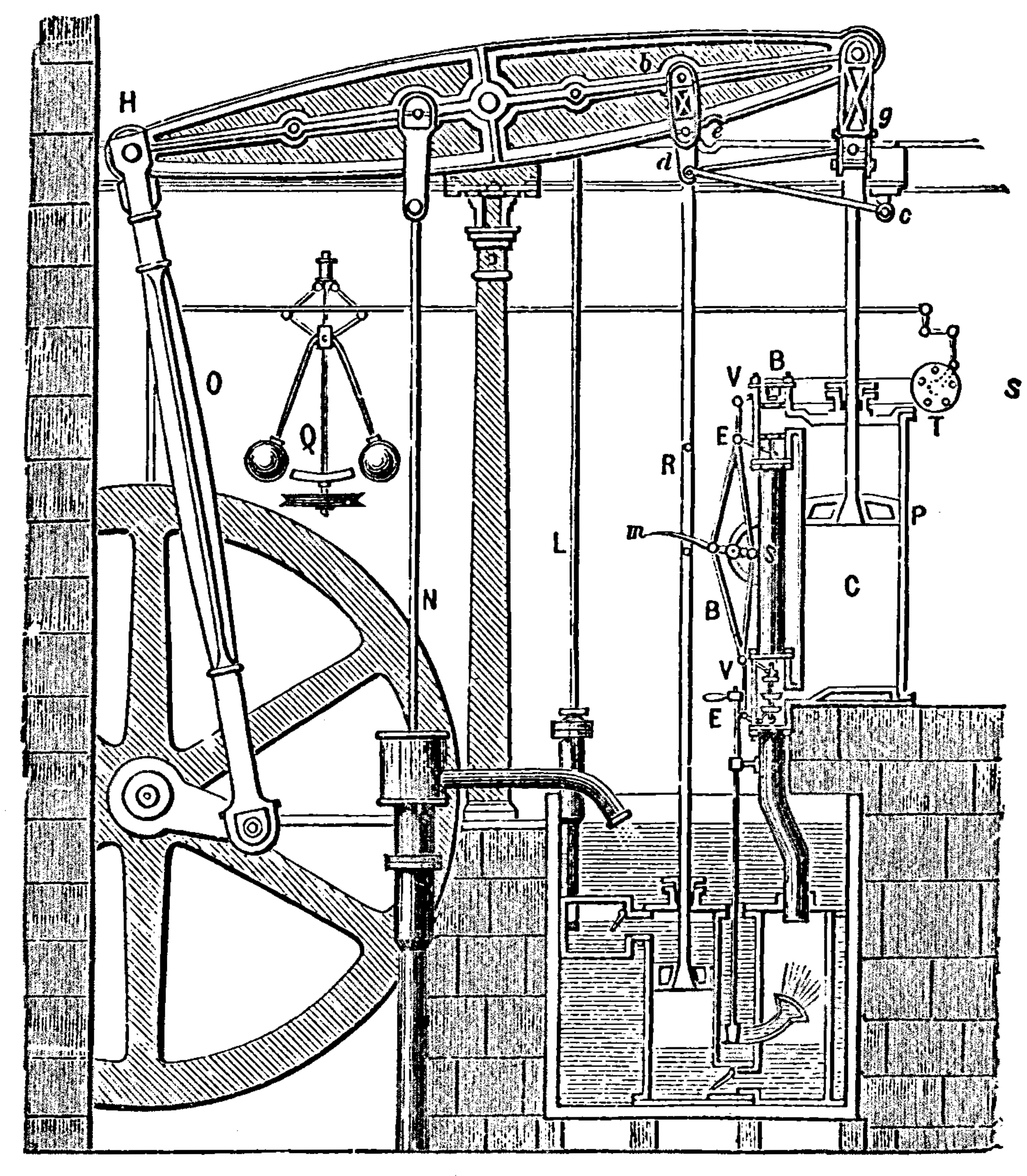
This was perhaps the first example of a controllable dynamical system.
Momentary and total payoff functions. We need to define a criterion that allows us to score or assign a real number to each candidate control function \(u\).
Suppose the momentary payoff—either a cost or reward—depends on time \(t\), the state of the system, \(x(t)\), and on a time-\(t\) selection of a control, \(u(t)\). We shall write this momentary payoff function as
The objective or criterion function that conveniently allows the decision maker to order and rank, or to discriminate between alternative controls, will be the sum of all momentary payoffs:
Example 11.2 (Reward function)
Suppose that \(h\) is a reward, utility or felicity function.
If we have two feasible alternatives \(u\) and \(u'\)—i.e., both satisfy (11.1)—then we say control function \(u\) is (weakly) better than \(u'\) if \(J(u) \geq J(u')\).
Notice that the example above is a comparison between two functions? We are deciding which of \(u\) or \(u'\) is better than the other. If we expand this idea, the general problem is one of selecting a particular function \(u\) that is best from some admissible set (\(U\)) of candidate control functions.
Definition 11.1 (Optimal Control Problem (FH-OCP))
Let \(T\) be a finite planning horizon and \(U\) be a non-empty, compact and convex set of functions.
The optimal control problem (OCP) beginning from initial data \((t_{0}, x_{0})\) is to select a function \(t \mapsto u(t)\) from \(U\) that satisfies the constraints in (11.1), such that it attains the highest possible value of the total payoff function (11.2).
That is, the OCP is the right-hand side of
and the value (indirect utility) of the optimal program beginning from \((t_{0}, x_{0})\) is the real number \(V(t_{0}, x_{0})\).
This is an infinite-dimensional problem, since the set \(U\) of such functions is an infinite set!
Can one mechanically set up a Lagrangian and solve a system of first-order conditions?
Fork in the road
Alas, there are uncountably and infinitely many such conditions.
Good luck trying to “solve” these like you would for finite-dimensional problems in your introductory optimization course!
So then you scratch your head and wonder: How does one manage this?
We will, figuratively and literally, find a path.
“The Russians [and the Americans (sic)] love their children too,” to paraphrase a Gordon Sumner lyric. Amidst post-WWII geopolitical shifts and the rise of the Cold War, two alternative ways of practically solving this hard problem were developed.
Roadmap
Section 11.3: We’ll begin our journey with a sufficient condition for optimality—the HJB equation. This is motivated by a very intuitive idea that if a plan or control is to be optimal, then any instantaneous action deviating from what is prescribed by the plan cannot deliver any total profit over the rest of the planning horizon. Along a particular path, the HJB equation also gives us the necessary conditions for optimality. Together, we have the BPO.
Section 11.5: Here, we will visit the Russian approach—the PMP formulation—that gives us the necessary conditions for optimal control. This will have vibes of the “Lagrangean-approach”, familiar to students who have taken a first course in convex optimization.
Section 11.6: We’ll make a connection between these two products of the Cold War and state under what conditions they are describing the same solution. We will see that this connection has a nice economic interpretation in terms of how we study general market equilibrium: Pareto (social) planner’s optimum versus decentralized (competitive) market equilibrium.
Section 11.7: We extend the treatment under a finite-horizon OCP to an infinite-horizon setting.
11.2. Bellman’s Principle of Optimality#
“A moment on the lips, a lifetime on the hips”, so says my annoying fitness coach Karen Mascador de Churros.
Let us take this outrageous hyperbole in for the moment.
(In some other plausible universe, this may also have been what Dicky Bellman’s mum said to him when he was a kid, with one arm halfway through the cookie jar.)
This little earworm will be the germ feeding our derivation of Bellman’s Principle of Optimality below.
Consider the finite-horizon OCP (11.3) with objective function (11.2).
Let’s pretend that we are able to compute this problem starting from some initial state \((t, x(t))\). If so, we would be able to work out the indirect utility \(V(t, x(t))\).
Of course, we don’t know the function \(V\) just yet. Have a little faith. We will get to the BPO insight for how to recover this \(V\)!
11.3. Sufficiency#
Our starting point is an intuitive criterion that is pure cost-benefit analysis:
Suppose a planner’s control \(u^{\ast}\) is optimal. For example, this plan says, “listen to your mum at all times, Dicky; suck in your lips and don’t let them near the cookies.”
Any temporary deviation from it, \(u(t) \neq u^{\ast}(t)\) would deliver an instance of gratification \(h(t, x(t), u(t))\). Think of this payoff as the marginal benefit of putting that cookie on your lips.
The marginal cost is our so-called “lifetime on your hips”—the negative of the rate at which the remaining total lifetime payoff changes—as a consequence of the deviation: \(-\dot{V}(t, x(t))\).
However, such a deviation must not be profitable over the remainder of your life. That is, the marginal variation to the (optimal) total value from this point on much be “costly enough” to enforce the correct incentive to “behave” according to \(u^{\ast}\):
Let \(\langle \cdot \rangle\) denote the inner-product operator.
We can write out (11.4) more verbosely:
This is often referred to as a Hamilton-Jacobi-Bellman (HJB) inequality.
We can check that this heuristic, a “one-shot deviation rule” or assumption, “makes sense”—i.e., it is indeed sufficient to enforce optimality.
Also, note the simplicity of this simple threat: One only needs to check that the consequence of one’s action \(u(t)\) satisfies this inequality at any given data point \((t, x)\)! Contrast this with the original OCP task of having to compare one control function, \(u\) against all others \(u'\) from an infinite set of such functions.
Integrating (11.5) with respect to \(t\) over the interval \([t_{0}, T]\), we have
The following creatures were exploited in the production of (11.6):
Since the OCP terminates in finite time \(T\), it is never optimal to derive any value from date \(T\) onwards: \(V(T, x(T)) = 0\).
The left-hand side (11.6) is the total lifetime payoff under any control policy \(u \neq u^{\ast}\). The right is the optimal value or indirect utility induced by sticking to \(u^{\ast}\), beginning from initial state \((t_{0}, x_{0})\).
That is, our point-wise heuristic (11.4) enforces the desired incentive.
If we re-arrange the inequality (11.5), we can see an alternative way to interpret (11.4):
This says that, the marginal cost induced by deviation \(u\) has to be at least as great as the sum of the instant gratification under \(u\) and its ensuing marginal lifetime benefit.
We can now work towards the sufficient HJB condition for solving the OCP (11.3):
Thus, if the control \(u^{\ast}\) were to be optimal, it must be that at each observed data point \((t,x)\), the selection \(u^{\ast}(t)\) renders the HJB inequality (11.7) binding—i.e., there is no incentive to deviate from this policy or control at any time and state:
(11.8)#\[\begin{split} \begin{split} -V_{t}(t, x) &= h(t, x, u^{\ast}(t)) + \langle V_{x}(t, x), f(t, x, u^{\ast}(t)) \rangle \\ &= \max_{k} \left\{ h(t, x, k) + \langle V_{x}(t, x), f(t, x, k) \rangle \right\}, \\ & \hfill \qquad\qquad\qquad\qquad\qquad\qquad\qquad\qquad \forall (t, x) \in [t_{0}, T] \times X. \end{split} \end{split}\]The last equality is by definition of an optimal policy. Equation (11.8) is a partial differential equation (PDE) which is called the Hamilton-Jacobi-Bellman (functional) equation.
This differential equation characterizes the solution for the function \(V\). Like all differential equations, it is a functional equation because the zero or the fixed-point of the equation is a (solution) function. Here that happens to be \(V: [t_{0}, T] \times X \rightarrow \mathbb{R}\) which has an economic meaning of an indirect utility function.
It is called a partial differential equation because unlike ordinary differential equations that involve partial derivatives of the solution with respect to time \(t\) (here, \(V_{t}\)), our PDE also involves partial derivatives of solution \(V\) with respect to other variables—the natural state of the controllable system \(x\). These partial derivatives are denoted by \(V_{x}\).
We can already see that the right-hand side maximization is a point-wise and low-dimensional problem, as opposed to an infinite-dimensional problem inherent in the original OCP (11.3).
Let \(\mu\) be a (technically, measurable) state feedback rule or function such that
(11.9)#\[ \mu(t,x) \in \text{arg}\max_{k} \left\{ h(t, x, k) + \langle V_{x}(t, x), f(t, x, k) \rangle\}\right\}, \]for all \((t, x) \in [t_{0}, T] \times X\), and, let \(x^{\ast}\) be a solution to the resulting IVP:
(11.10)#\[ \dot{x}^{\ast}(t) = f\left(t, x^{\ast}(t), \mu(t, x^{\ast}(t))\right), \ x(t_{0}) = x_{0}, \]for all \(t \in [t_{0}, T]\). Then \(\mu(t,x^{\ast}(t)) = u^{\ast}(t)\).
Combining the last point in the HJB Equation (11.8) and then integrating it over the interval \([t_{0}, T]\), we get
\[ 0 = \int_{t_{0}}^{T}h(t, x^{\ast}(t), u^{\ast}(t)) + V(T, x(T)) - V(t_{0}, x_{0}). \]Since it is never optimal to derive any value beyond the terminal date, then \(V(T, x)=0\) for any \(x\), and we have
(11.11)#\[ V(t_{0}, x_{0}) = \int_{t_{0}}^{T}h(t, x^{\ast}(t), u^{\ast}(t)) \equiv J(u^{\ast}). \]Suppose without loss of generality, \(t_{0}=0\). By the last three parts, \(V(t', x')\) is the optimal value of OCP (11.3) with initial data \((t', x') \in\ (0,T] \times X\) and it is unique by construction. Since \(V\) is continuous on \([0,T] \times X\), then for all \((t,x) \in [0,T] \times X\), \(V(t,x)\) is unique. Uniformly, there is a unique function \(V: [t_{0}, T] \times X \rightarrow \mathbb{R}\) solving the HJB equation.
Theorem 11.1 (HJB Equation)
Let \(V: [t_{0}, T] \times X \rightarrow \mathbb{R}\) be a continuously differentiable function which solves the HJB equation (11.8) for all \((t, x) \in [t_{0}, T] \times X\) along with the boundary value \(V(T, x) = 0\).
Then a measurable function \(\mu\) satisfying (11.9)—which attains the maximum on the RHS of the HJB Equation such that the (11.10) holds—must be the optimal control: \(\mu(t,x^{\ast}(t)) = u^{\ast}(t)\).
This optimal control delivers the same optimal value as the original OCP (11.3).
That is, solving the partial differential or HJB equation (11.8) for the unique \(V: [t_{0}, T] \times X \rightarrow \mathbb{R}\) suffices for solving the OCP (11.3).
Bellman’s Principle of Optimality
The HJB equation (11.8) gives us the insight of Bellman’s Principle of Optimality (BPO).
Regardless of how one arrived at the initial data \((t, x)\), the optimal policy \(\mu(t,x) = u^{\ast}(t)\) tells us that it is independent of \(x\). It only requires that all subsequent actions are selections from the optimal control. That is, they are optimal.
This implies the optimal policy can be obtain by backward induction, working backwards from the end where \(V(T, x) = 0\).
Exercise 11.1 (Linear optimal regulator)
Consider a linear controllable system, where \(x \in X \subset \mathbb{R}\).
(Note that \(f\) here turns out to be time invariant.)
Suppose the OCP now has an objective function that involves discounting of future payoffs and the discount rate is \(r \geq 0\). For any \(t_{0} \geq 0\), the present discounted value of the objective function is:
where
(Setting \(r=0\) would be akin to the undiscounted OCP earlier.)
Write down the HJB equation that characterizes the solution for the (unknown) value or indirect-utility function \(V\).
Hint: Guess that the solution has a quadratic form \(V(t,x) = -Q(t)x^{2}\). Also we have \(V(T,x) = 0\) as a terminal boundary value.
You can solve this particular PDE, but the PDE is a nonlinear differential equation in \(Q(t)\).
Hint: Define a change of variables \(Q(t) = Z(t)/Y(t)\) and transform the equation into a two-variable linear ODE system in \((Y, Z)\).
Show that the optimal state feedback decision rule \(\mu(t, x)\) is linear in the state \(x\).
Derive the optimal path of the state variable, \(x^{\ast}(t)\) induced by the optimal linear regulator \(\mu(t, x)\).
Derive the optimal control path \(u^{\ast}(t) = \mu(t, x^{\ast}(t))\).
11.4. HJB, BPO and Necessity#
OK, so if we can solve the PDE that is the HJB equation, then that suffices to solve the original OCP (11.3).
In practice, PDEs do not always have convenient closed-form solutions.
Also, note that solving the PDE means solving for a function \(V\) as a fixed point of the HJB functional equation (11.8). That is we need to evaluate the HJB equation for all \((t, x) \in [t_{0}, T] \times X\)! Computationally, this can be quite expensive when \(x\) is a vector of state variables.
What if we are interested in the local properties of the HJB equation, within the neighborhood of a solution to the original (11.3)?
That is, the HJB equation and therefore BPO will also provide us with the necessary conditions for optimality.
Here’s how this works. From Theorem 11.1, we know that the HJB equation suffices for optimality. Therefore, the optimizer in (11.9) at each date-state pair—i.e., the control feedback outcome \(\mu(t, x)\)—is attaining the maximum on the right-hand side of (11.8) or (11.9).
Along the optimal path, i.e., evaluating at \(\mu(t, x)\), the marginal value of the objective function in the right-hand side of (11.8) with respect to state \(x\) is:
for all \((t, x) \in [t_{0}, T] \times X\). The last line follows from the Envelop Theorem applied to the HJB equation along an optimum.
Likewise, along the optimum, if we differentiate (11.8) with respect to \(t\), we get
for all \((t, x) \in [t_{0}, T] \times X\).
To the sleepy cat, this looks like a complicated ball of yarn. Before you get too lippy about it, let’s recall our hyperbole on lips and hips.
Equations (11.12) and (11.13) necessarily describe the optimal control path. Here’s how to read these conditions:
Holding our position fixed at \((t,x)\) along the optimal path, what if we perturbed the optimal path a little by perturbing the current state \(x\)? Think of \(x\) as wealth or capital, if you need a concrete example.
Equation (11.12) tell us how that small variation in \(x\) contributes to an instantaneous marginal benefit, \(h_{x}(t,x,\mu(t,x))\), and how that is necessarily balanced by a variation in the continuation marginal cost from the immediate moment thereafter, i.e., the terms \(-\left[ \dot{V}_{x}(t,x) + V_{x}(t,x)f_{x}(t, x, \mu(t,x))\right]\).
There are two terms here since a perturbation in \(x\) affects the rate at which the optimal marginal value changes over time directly and it also affect the continuation marginal value through the transition law of the state (\(f\)).
That is, we have an intertemporal trade-off in how to use or eat into our wealth \(x\)!
You can similarly interpret a trade-off in the second condition (11.13).
Exercise 11.2
Interpret the necessary condition in Equation (11.13).
Together (11.12) and (11.13) give us the necessary dynamic trade-offs involved when we “explore”—in (the state) space and across time—within a small neighborhood around a point \((t,x)\) on the optimal path.
11.5. Pontryagin’s Maximum Principle#
If we are not immediately interested in directly solving the HJB equation, the necessary conditions under Pontryagin’s Maximum Principle (PMP) will turn out to be easier to analyze.
Let’s see why.
Let us define an intermediate objective function called the Hamiltonian:
Can you see that the animal on the right-hand side of (11.14) is suspiciously similar to the objective in the curly braces of Equation (11.9)? (You might think we’re painting stripes on a skinny dog to pass it off as a Tasmanian tiger.)
Our Trojan horse here is brought to you by the Greek letter \(\psi\).
The Hamiltonian (11.14) has economic meaning. For concreteness, consider the example where \(u(t)\) is consumption and \(x(t)\) is capital stock or wealth. Then, we can see that at each moment in time, the decision maker’s choice of \(u(t)\) impacts on the value the Hamiltonian (“rate of change of total utility”) directly, through the instantaneous payoff term \(h(\cdot)\).
This choice also affects the Hamiltonian indirectly, through influencing future consumption opportunities and thus utility (Hamiltonian value) by altering the transition to future states (of wealth). This indirect effect is captured by the inner-product term on the right of (11.14). The function \(t \mapsto \psi(t)\) is the shadow price of this constraint, that translates the effect of \(u\) on future states (via \(\dot{x}\)) into “utility terms.”
In PMP’s formulation, if \(t \mapsto \psi(t)\) can be suitably chosen, then the value of this shadow-pricing function would align with the planner’s marginal value of initial wealth, \(V_{x}(t,x(t))\), along the optimal path.
More precisely, if the adjoint or co-state variables \(\psi(t)\) and \(\psi^{0}(t)\) were chosen such that \(\psi(t) = V_{x}(t, x^{\ast}(t))\) and \(\psi^{0}(t) = V_{t}(t, x^{\ast}(t))\), we can verify that the necessary condition (11.12) implies the adjoint equation:
and the boundary condition \(V(T,x) = 0\) for all \(x\) implies the transversality condition:
The maximization on the right-hand side of Equation (11.9) implies:
Lastly, (11.13) implies the maximized Hamiltonian:
This provides the envelop condition
Proposition 11.1 (Pontryagin Maximum Principle (FH-OCP))
Given a state-control trajectory \(\left(x^{\ast}(t), u^{\ast}(t)\right)\), \(t \in [t_{0}, T]\), solving the original OCP (11.3), there is an absolutely continuous function \(t \mapsto \psi(t)\) such that these conditions necessarily hold:
Adjoint equation: (11.15);
transversality condition: (11.16);
maximality: (11.17); and
envelop condition: (11.19).
The optimal trajectory of the state is
for all \(t \in [t_{0}, T]\).
Stare at these conditions and think for a bit. We’ll see that the system given in Equations (11.15)—(11.19) and (11.20) is an ordinary differential equation system in \((\psi, x, u)\).
In practice, we can solve these ODEs by integration (or point-wise numerical integration). If not, we can at least analyze the dynamic behavior qualitatively (if the system is low dimensional enough).
11.6. Duality: Resource prices and planner’s marginal valuation#
“The stripey skinny dog is the Tassie Tiger!” shrieks Dicky. Under some conditions.
Mantra of the day
Solving the HJB equation implies maximizing the associated Hamiltonian.
Maximizing a Hamiltonian does not always imply solving the same optimal control under the HJB equation.
Read the statement of the PMP—Proposition 11.1—again. It says that given an optimal state-action trajectory solving the planners’ OCP, there exists a shadow-pricing function \(\psi\) that could be chosen such that the PMP necessary conditions may align with the HJB equation. (Recall that the HJB equation and its associated state-feedback optimal regulator \(\mu\) suffice to attain the planner’s optimal solution.)
In other words, the HJB equation implies maximizing the associated Hamiltonian, but not necessarily vice-versa.
Later, when we consider models with market solutions—where allocations are “decentralized” through a Walrasian pricing mechanism—and contrast them with their respective social-planer’s allocation, the comparison between HJB and PMP will pop up again. Students who have internalized lessons from general equilibrium theory would see the similarity here to the First- and the Second Fundamental Welfare Theorems in general equilibrium.
The HJB sufficiency and necessity results (Theorem 11.1 and Proposition 11.1) can be compared to the Second Welfare Theorem in the sense that if the shadow-pricing function \(\psi\) aligns with the planner’s marginal value function, then the PMP formulation (read, competitive equilibrium) is equivalent to the HJB formulation (read, Pareto optimum).
The reverse statement need not always be true, just as in the First Welfare Theorem. We may have competitive equilibria that may not be Pareto optimal. In the dynamic setting, this will show up as solving a Hamiltonian where the solution, if it exists, may result in pricing functions that are not necessarily aligned with the planner’s optimal marginal valuation.
Thus, the equivalence between PMP and HJB does not come for free. With additional concavity restrictions on the Hamiltonian function, we can ensure that the necessary PMP conditions are also sufficient (i.e., PMP is equivalent to the HJB):
Proposition 11.2 (Mangasarian Sufficiency Theorem)
Consider a state-control trajectory \(\left(x(t), u(t)\right)\), \(t \in [t_{0}, T]\), for the OCP (11.3).
If \(H(t,x,u,\psi)\) is concave in \((x,u)\) and there is
an absolutely continuous function \(\psi: [t_{0}, T] \rightarrow \mathbb{R}^{n}\) such that the adjoint equation (11.15) holds,
\(\psi(T) = 0\), and,
maximality (11.17) holds,
then \(\left(x(t), u(t)\right) = \left(x^{\ast}(t), u^{\ast}(t)\right)\), \(t \in [t_{0}, T]\) is an optimal state-control path.
Additionally, if \(H(t,x,u,\psi)\) is strictly concave in \((x,u)\), then the optimal state-control path is unique.
Remark 11.1
Condition 1 in Proposition 11.2 holds if the primitive functions \(h\) and \(f\) are concave in \((x,u)\).
Exercise 11.3 (Finite-horizon Ramsey Problem)
Consider the model of capital production:
where \(d\) represents the effective drag or depreciation on growth in the capital stock \(k\) and \(c(t)\) is consumption outcome at time \(t\). If you need to be explicit, you may assume the production function is Cobb-Douglas: \(\phi(k) = k^{\alpha}\) and \(0<\alpha<1\).
(Note that in this application, the controllable state-transition map, \(f\), is a time-invariant function.)
Suppose the momentary payoff is \(h(t, k, c) \equiv\ h(c)\), i.e., it is a time-invariant and state-independent function. The planner’s objective function is
where \(\rho>0\) is the planner’s subjective rate of time preference (or preference-driven discount rate). If you crave specifics, you may also assume \(h(c) = \ln(c)\).
The planning problem of maximizing (11.22) by choosing an optimal control \(c: [0,T] \mapsto \mathbb{R}_{++}\), is subject to (11.21), the boundary values \(k(0) = k_{0} > 0\) and \(k(T) = k_{T} \geq 0\). The value \(k_{T}\) is an end-point that can be freely chosen.
Assume that \(h' > 0\), \(h'' <0\); \(\phi' > 0\), \(\phi'' < 0\), \(\phi(0)=0\) and the usual Inada conditions hold for \(h\) and \(\phi\). Also assume that \(\lim_{k \nearrow \infty} \phi'(k) < \rho + d < \lim_{k \searrow 0}\phi'(k)\).
Define the optimal control problem (OCP) for this application.
Construct the HJB equation defining the planner’s optimal state-control path. Explain what this says in the context of the example and why this equation has potentially practical usage.
If a state-control path solves the OCP, derive the necessary conditions governing the path’s optimality from the HJB formulation.
Define the Hamiltonian for the PMP formulation of this problem. Use \(\psi(t)\) to represent the adjoint variable or multiplier on the state-transition constraint (11.21).
Show that the solutions to the problems, HJB and PMP, are the same. Why are they the same?
What can you learn from these necessary and sufficient conditions for optimal saving?
Note: In this example, there is only one state variable, so inner-product notations would just be the same as scalar multiplication operators.
11.7. Discounted programming and the infinite horizon#
In practice one might argue there is no such thing as an infinite horizon. The lazy antagonist would even invoke the hackneyed Keynesian quote: “In the long run we are all dead.”
So then why consider modelling optimal control problems with an infinite planning horizon?
With finite-horizon, there is an end-of-horizon effect on the optimal plan. Big \(T\) affects incentives.
For example, when one’s model of optimal fishing has a finite horizon, one gets the absurd and dismal result that at the end, at time \(T\), one just completely exhausts the stock of fish in the lake or ocean! This may not be a desirable feature if one has an ongoing concern about the resource.
Taking \(T \rightarrow \infty\) is our modeller’s metaphor for this ongoing concern. It is not literally that one lives forever.
Definition 11.2 (Infinite-horizon Optimal Control Problem (IH-OCP))
Let \(T \rightarrow \infty\) define the infinite planning horizon and \(\Gamma\) be a non-empty, compact and convex set. Let the total-payoff objective function, with \(T \rightarrow \infty\) and \(h\) no longer depends on \(t\), be:
The infinite-horizon optimal control problem (hereinafter, also OCP), beginning from initial data \((t_{0}, x_{0})\), is to select a function \(t \mapsto u(t)\) from \(U\) that satisfies the constraints in (11.1), such that it attains the highest possible value of (11.23).
That is, the infinite-horizon OCP is the right-hand side of
and the value (indirect utility) of the optimal program beginning from \((x_{0})\) is the real number \(V(x_{0})\).
Compared to (11.3) earlier, observe that we have now dropped the dependence of functions \(h\), \(f\) and therefore \(V\) on time \(t\). Intuitively, this is because as one takes \(T \rightarrow \infty\), the “end” or the big \(T\), no longer has bite. Formally, one can also show that the infinite set of functions \(V(t, x)\) indexed by \(t\) would converge to a time-invariant limit \(V(x)\) and so the optimal state-feedback rule \(\mu(t,x)\) should also converge to a time-variant function \(\mu(x)\). This is beyond the level of this course.
The HJB equation for \(T \rightarrow \infty\) simplifies a lot:
The PMP necessary conditions are the same:
Adjoint equation: (11.15);
transversality condition (below) (11.26);
maximality: (11.17); and
envelop condition: (11.19).
The difference now is that there is no determinate terminal condition. One might expect this to be a “natural” transversality condition:
This has the meaning that into the very indefinite future, the (present-value) shadow price of the state—wealth, for example—should go to zero.
However, this may not always hold in all models/problems. An alternative infinite-horizon transversality condition would be
This has an economic interpretation: The value of the state (i.e., of accumulating wealth) into the indefinite future must be asymptotically zero. Otherwise, one always “leaves something behind” forever. Note that, if the state \(x(T)\) grows forever, then its shadow price must tend to zero at a faster rate.
So you might ask: Is there a definitive transversality condition? The short answer is one has to approach the problem with brains on: Think about what is “natural” and “meaningful” for your problem.
11.8. Remarks#
As promised, this is a quick review and not a comprehensive one. Most economics textbook treatment of the PMP take a more procedural approach. Here, we have tried to strike a balance between providing the cookbook recipes and the original thinking that led to such recipes. That is, our treatment here aimed at providing a bit more foundation for the PMP, beginning from a BPO perspective. This follows the lead of Weber [33]. We added more verbal exposition and economic reasoning to the key insights for the BPO.
We made an intuitive jump in the infinite horizon setting by just stating how the problem can be constructed. We also just pointed out what needed to be modified relative to the finite-horizon setting. We also omitted the generalization of the BPO and PMP to problems where there are additional state-control contraints. Also, we skipped the proof of the PMP altogether. The reader keen on getting into the guts of these topics can work through more material in Weber [33], for example. Léonard and Ngo [15] provide a slightly more reader-friendly and casual treatment on this subject.