13. Solving an example Ramsey-Cass-Koopmans Model#
Let
capital stock per efficiency units of worker be \(k := k(t)\); and,
consumption per efficiency units of worker be \(c := c(t)\).
Also, we have:
Capital depreciation rate: \(\delta \in (0,1]\);
population growth rate: \(n \in [0,\infty)\); and,
rate of technological progress: \(g \in [0,\infty)\).
The model’s Pareto optimum—or equivalently, competitive equilibrium—is characterized by a pair of differential equations determining the solution functions \(t \mapsto (k(t), c(t))\) and boundary values:
Resource constraint
\[ \dot{k} = f(k) - (n+g+\delta)k - c. \]The Euler-Lagrange equation (or Keynes-Euler rule)
\[ \frac{\dot{c}}{c} = \frac{1}{\sigma(c)} \left[ f'(k)-(\delta+\rho+\sigma g) \right] \]where \(\sigma(c) = u''(c)c/u'(c)>0\) is the relative risk aversion (RRA) coefficient.
Boundary values
\[ k(0) = k_{0}, \qquad \lim_{T\rightarrow\infty}e^{-\rho T}u'(c(T))k(T) = 0. \]
We will work with the special case:
Constant RRA (or CRRA) preferences where \(\sigma(c) = \sigma\); and
Cobb-Douglas production where \(f(k) = k^{\alpha}\) and \(\alpha \in (0,1)\).
Conditions 1 and 2 above imply a differential operator
13.1. BVP as IVP#
Notice that the system above has no initial condition on \(c(t)\).
It is a “jump” variable.
We can show that the system above has a unique, nontrivial steady state \(\bar{k} \in (0,\infty)\) that is a locally saddle-path stable.
The original problem is an infinite-horizon program. In our numerical implementation, we will have to approximate this with a finite horizon approximant: When we solve the system below we have to terminate the integration in finite steps.
Theoretically, we know that the solution will be saddle-path stable, so we expect the solution to converge to the steady-state equilibrium for a large-enough horizon \(T\). As such, we will replace the boundary values above with
\(k(0) = k_{0}\) and \(k(T) = \bar{k}\).
This boundary-value problem, denoted as BVP-\((k_0, \bar{k})\), can be re-cast as an initial value problem, IVP-\((k_0, c(0))\).
This is a standard trick in solving BVPs. See this video for a quick review or refresher!
The task will be as follows:
Find an appropriate guess of the jump \(c(0) = c_0\).
Solve IVP-\((k_0, c(0))\) to get a trajectory \(\mathbf{k}(c_0, k_0) = \{ k(t,c_0): k(0) = k_0, t\in[0,T]\}\) for some large enough horizon \(T\).
We require that the guess \(c_{0}:=c_{0}(k_{0})\) yields \(k(T,c_0) = \bar{k}\). That is, we choose \(c_0\) to satisfy the zero of
\[ e(c_0; \bar{k}, T) := k(T,c_0) - \bar{k}. \]
import numpy as np
import matplotlib.pyplot as plt
from scipy.integrate import solve_ivp
# Define model bits
def f(k, α):
    """Cobb-Douglas production function f.
    Returns output per efficient worker."""
    return k**α

def fprime(k, α):
    """Cobb-Douglas f's MPK"""
    return α*k**(α-1.0)

def T(t, state, ρ, σ, n, g, δ, α, β):
    """Equilibrium operator T: The ODE system.
    Here, c is a jump variable, but we'll call it
    a state for the purposes of this T map. When
    we integrate T, this will be a BVP with two boundary
    values. We can re-state the BVP as an IVP with a
    correct guess of the jump c(0)."""
    k, c = state[0], state[1]
    kdot = f(k, α) - (n + g + δ)*k - c
    cdot = (fprime(k,α) - (δ + ρ + σ*g))/(σ*c)
    return [kdot, cdot]

def steadystate(ρ, σ, n, g, δ, α, β):
    """Steady state equilibrium"""
    kss = (α/(δ + ρ + σ*g))**(1.0/(1.0-α))
    css = f(kss, α) - (n + g + δ)*kss
    return kss, css

def c_kdotzero(k, n, g, δ, α):
    return f(k, α) - (n + g + δ)*k

def T_zero(k, ρ, σ, n, g, δ, α, β):
    """Two loci of (k,c) pairs such that
    (1) dk/dt = 0, or
    (2) dc/dt = 0;
    i.e., T(x) ≡ (T_k, T_c)(x) = 0.
    """
    # kdot = 0 locus
    h_kdotzero = f(k, α) - (n + g + δ)*k
    # cdot = 0 locus
    css = steadystate(ρ, σ, n, g, δ, α, β)[1]
    h_cdotzero = np.linspace(0.0, css*2.0, k.size)
    return h_kdotzero, h_cdotzero
13.1.1. Secant method for root finding#
Let’s take a quick detour here to discuss the root-finding problem in our shooting algorithm.
For the root-finding part, we’ll use a derivative-free approach known as the secant method.
You can also try the bisection method which converges at a slower, linear rate.
To motivate the use of such an algorithm, let’s put on our analytical thinking caps.
From elementary analysis, we know that there is a unique root for any continuous and monotone function on a bounded domain.
In practice, as is here, the solution \(k(\cdot,c_0)\) is endogenous, and to us, it is an unknown function: We also don’t have an analytical solution form.
Thus, for a fixed horizon \(T\) and target end-point \(\bar{k}\), we may not know a priori whether the function \(e(c_0; \bar{k}, T)\)—whose root in terms of \(c_0\) we must find—is continuous and monotone in the initial jump \(c_0\).
However, this model is tractable enough locally:
We can deduce that an equilibrium (or optimal) trajectory will be along a saddle-path stable arm and the stable arm—or the solution curve, \(k(t,c_0)\) for every \(t\)—will be monotone in \(c_0\) if \(c_0\) is not too far away from the exact \(c_0(k_0)\) that is on the stable arm.
We can deduce all this by bothering with the phase diagram analysis!
Since \(e\) is linear in \(k(T,c_0)\) then \(e(c_0; \bar{k}, T)\) will be continuous and monotone in \(c_0\) too, for some small set \([\underline{c}_{0}(k_{0}), \overline{c}_{0}(k_0)]\) containing the guess \(c_0\).
We should expect the set \([\underline{c}_{0}(k_{0}), \overline{c}_{0}(k_0)]\) to be shrinking the further the initial state \(k_{0}\) is away from the steady state point \(\bar{k}\).
def secant_method_recursion(f, x_min, x_max,
                          iteration=0, TOL=1e-5,
                          MAXITER=200, verbose=True):
    """Secant method for root finding of a
    continuous scalar function on a bounded
    domain. Convergence rate faster than
    bisection's linear rate."""
    if verbose and iteration==0:
        print("Iter \t x \t f(x)")
    # Function values at domain limits
    y0, y1 = f(x_min), f(x_max)
    # Next best root approximant:
    # inverse of affine map
    x_new = x_max - y1 * ((x_max - x_min) / (y1 - y0))
    # check tolerance condition
    if -TOL < y1 < TOL:
        print("Converged!\n")
        return x_new, f(x_new), iteration
    else:
        x_min = x_max
        x_max = x_new
    if verbose:
        print("%i \t %4.3f \t %4.3f"
                %(iteration, x_new, y1))
    iteration += 1
    if iteration < MAXITER-1:
        return secant_method_recursion(f, x_min, x_max,
                                     iteration=iteration)
    else:
        print("WARNING: MAXITER reached!")
        return x_new, f(x_new), iteration
Let’s put our bespoke code above to the test:
Find the unique root of \(\sin(x)\) for \(0<x<2\pi\)
x = secant_method_recursion(np.sin,
                            np.pi/2.0+0.01, 1.4*np.pi,
                            MAXITER=20)
Iter 	 x 	 f(x)
0 	 3.025 	 -0.951
1 	 3.175 	 0.117
2 	 3.142 	 -0.033
3 	 3.142 	 0.000
Converged!
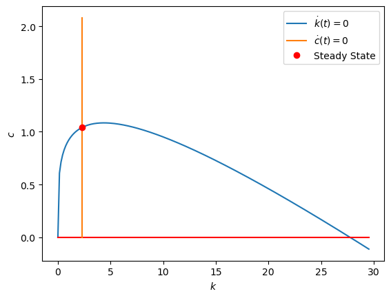
13.2. Nullclines and phase plot#
def plot_nullclines(plt, k_grid, h_kzero, h_czero, kss):
    """Plot two sets of (k,c) pairs such that
    (1) dk/dt = 0, or
    (2) dc/dt = 0
    """
    plt.xlabel(r"$k$")
    plt.ylabel(r"$c$")
    plt.plot(k_grid, h_kzero, label=r"$\dot{k}(t)=0$")

    plt.plot(k_grid, 0.0*k_grid, '-r')
    plt.plot(kss*np.ones(h_czero.size), h_czero, label=r"$\dot{c}(t)=0$")
    plt.plot(kss, css, 'or', label="Steady State")
    return plt
Let’s evaluate a parametric instance of the model:
# Parametric instance
ρ = 0.05
σ = 3.0
n = 0.001
g = 0.0017
δ = 0.08
α = 0.25
β = 0.5
This instance yields the steady state equilibrium point:
# Solve for steady state
kss, css = steadystate(ρ, σ, n, g, δ, α, β)
print("Steady state equilibrium")
print("kss = %1.5g, css = %1.5g" %(kss, css))
Steady state equilibrium
kss = 2.2718, css = 1.0398
Now let’s compute this model instance’s nullclines and visualize them in \((k,c)\)-space:
# Consider zooming into neighborhood around steady state
# Grids of k and c
N_grid = 200
kmin, kmax = 0.0*kss, 13.0*kss
k_grid = np.linspace(kmin, kmax, N_grid)

# Nullclines are N_k ≡ (k_grid, h_kdotzero) and N_h ≡ (k_grid, h_hdotzero)
h_kdotzero, h_cdotzero = T_zero(k_grid, ρ, σ, n, g, δ, α, β)
# Show nullclines

plt.figure()
plt = plot_nullclines(plt, k_grid, h_kdotzero, h_cdotzero, kss)
plt.legend();
Next, we want to study the solution behavior (equilibrium dynamics) using a phase diagram:
def phaseplot(plt, k_grid, c_grid,
                        alpha=0.5,
                        norm_grad=False):
    """Plot vector field elements: gradient vectors"""
    X, Y = np.meshgrid(k_grid, c_grid)
    X = X.flatten()
    Y = Y.flatten()
    # Rates of change from ODE
    state = [X, Y]
    dx, dy = T(None, state, ρ, σ, n, g, δ, α, β)

    if norm_grad:
        # Normalize these vectors
        # Hide true magnitude
        norm = np.sqrt(dx**2. + dy**2.)
        U = dx / norm
        V = dy / norm
    else:
        # Un-normalized gradient vectors
        # Shows magnitude!
        U = dx
        V = dy

    # Plot vector field
    plt.quiver(X, Y, U, V, angles='xy', alpha=alpha)
    # Grid lines for visual ease
    plt.grid()
    return plt
# Get the grid space for c to be of the same limit as that
# implied by the plotted nullclines

# A sparser grid of k for plotting gradient vectors
N_gradvecs = 23
k_spgrid = np.linspace(0.001, k_grid.max(), N_gradvecs)

# Lower bound of plot
cmin = 0.05

# Upper bound of plot
cmax = max([h_kdotzero.max(), h_cdotzero.max()])

# (Sparser) grid of c
c_spgrid = np.linspace(cmin, cmax, k_spgrid.size)
plt.figure()
plt = plot_nullclines(plt, k_grid, h_kdotzero, h_cdotzero, kss)
plt = phaseplot(plt, k_spgrid, c_spgrid,
                        alpha=0.3,
                        norm_grad=True)
plt.legend();
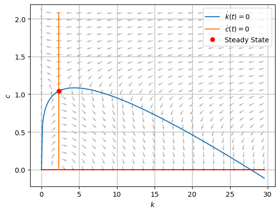
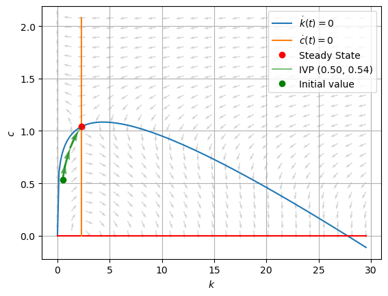
As we have deduced earlier using pencil and paper, the vector field suggests that there is a saddle-path stable arm that describes the solution curve.
13.3. Shooting algorithm and solution curve#
Now we turn to the task of numerically computing the solution curve.
We can re-cast the original BVP-\((k_0,\bar{k})\) as an IVP-\((k_0, c(0))\) by
Guessing a jump \(c(0) = c_0\)
Ensuring solution \(\mathbf{k}(c_0, k_0) = \{ k(t,c_0): k(0) = k_0, t\in[0,T]\}\) yields \(e(c_0; \bar{k}, T) = k(T,c_0) - \bar{k}=0\).
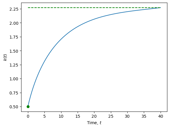
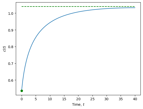
13.3.1. Trajectory from \(k(0) < \bar{k}\)#
# Time domain to perform integration
t_min = 0.0
t_max = 40.0
t_span = [t_min, t_max]

# Finer mesh to evaluate solution curve
t_eval = np.linspace(t_min, t_max, 100)

# Initial state
k0 = 0.5
# Solution path, terminal state k(T; c0) as function of c0
# We define this easy to use function in a few steps to account
# for some solution paths that may "blow up".

def trajectory(c0, k0, kss, T_operator, t_span,
               args=(ρ, σ, n, g, δ, α, β),
               method='Radau'):

    sol = solve_ivp(T_operator, t_span, [k0, c0],
                          method=method,
                          args=args
                          )
    kT = sol.y[0][-1]
    return kT

# Define error function, whose zero is the solution c0
errfun = lambda c0: trajectory(c0, k0, kss, T,
                               t_span, args=(ρ, σ, n, g, δ, α, β)) - kss
# Small interval containing guess of initial jump c0
c_lo = 0.52
c_hi = 0.536358

# Use secant root-finder to update guess of c0
c0_jump, fval, iteration = secant_method_recursion(errfun,
                                                   c_lo, c_hi)

print("c0 = %6.12g" % (c0_jump))
print("errfun(c0) = %6.12g" % (fval))
print("Total iterations = %i" % (iteration))
Iter 	 x 	 f(x)
0 	 0.534 	 -1.320
1 	 0.536 	 4.866
2 	 0.536 	 1.154
3 	 0.536 	 -2.182
4 	 0.536 	 0.420
5 	 0.536 	 0.155
6 	 0.536 	 -0.013
7 	 0.536 	 0.000
Converged!

c0 = 0.53615456467
errfun(c0) = 5.05302022447e-10
Total iterations = 8
# Initial value of state
x0 = [k0, c0_jump]

# Integrate ODE - use SciPy's SOLVE_IVP
def event_ss(t, state, ρ, σ, n, g, δ, α, β):
    """Return t's where dk/dt = T(t, state) ≈ 0.
    That is, we are at steady state."""
    return T(t, state, ρ, σ, n, g, δ, α, β)[0]

event_ss.direction = -1
event_ss.terminal = True

psol = solve_ivp(T, t_span, x0,
                 method='Radau',
                 args=(ρ, σ, n, g, δ, α, β),
                 events = [event_ss,],
                 t_eval=t_eval,
             )
# # Show gradient on particular solution curve
ut, vt = T(None, psol.y, ρ, σ, n, g, δ, α, β)
norm = np.sqrt(ut**2. + vt**2.)
ut = ut/norm
vt = vt/norm

# Sample gradient vectors
select = (np.ceil(t_max/np.array([t_max, 8, 2]))).astype(int).tolist()

plt.figure()
plt = plot_nullclines(plt, k_grid, h_kdotzero, h_cdotzero, kss)
plt = phaseplot(plt, k_spgrid, c_spgrid,
                        alpha=0.175,
                        norm_grad=True)
# Particular solution for IVP
plt.plot(psol.y[0], psol.y[1], '-g', alpha=0.5,
            label="IVP (%0.2f, %0.2f)" % (x0[0], x0[1])
        )
plt.quiver(psol.y[0][select], psol.y[1][select],
            ut[select], vt[select],
                angles='xy', alpha=0.65, pivot="mid",
                            width=0.0061, color="green")
plt.plot(x0[0], x0[1], 'og', label="Initial value")
plt.legend();
Let’s view this solution curve in terms of a time path or trajectory:
# Time path of solution, k(t), c(t)
variables = [r"$k(t)$", r"$c(t)$"]
steady = [kss, css]

for idx, var in enumerate(variables):
    plt.figure()
    plt.plot(t_eval, psol.y[idx])
    plt.plot(t_eval[0], x0[idx] ,'og')
    plt.plot(t_eval, steady[idx]*np.ones(t_eval.shape),
                                    '--', color="green")
    plt.xlabel(r"Time, $t$")
    plt.ylabel(var);
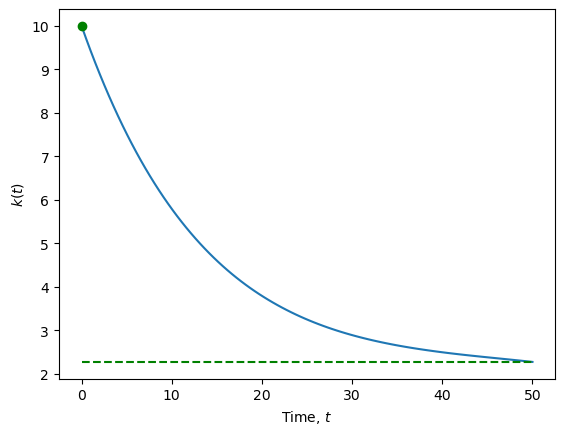
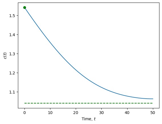
13.3.2. Trajectory from \(k(0) > \bar{k}\)#
t_max = 50.0
t_span = [t_min, t_max]
# Finer mesh to evaluate solution curve
t_eval = np.linspace(t_min, t_max, 100)
# Define error function, whose zero is the solution c0
k0 = 10.0
errfun = lambda c0: trajectory(c0, k0, kss, T,
                               t_span, args=(ρ, σ, n, g, δ, α, β)) - kss
# Small interval containing guess of initial jump c0
c_lo = 1.4881
c_hi = 1.5432
# Use secant root-finder to update guess of c0
c0_jump, fval, iteration = secant_method_recursion(errfun,
                                                   c_lo, c_hi)

print("c0 = %6.12g" % (c0_jump))
print("errfun(c0) = %6.12g" % (fval))
print("Total iterations = %i" % (iteration))
Iter 	 x 	 f(x)
0 	 1.533 	 -2.172
1 	 1.540 	 4.122
2 	 1.543 	 1.350
3 	 1.541 	 -1.571
4 	 1.541 	 0.350
5 	 1.542 	 0.091
6 	 1.542 	 -0.006
7 	 1.542 	 0.000
Converged!

c0 = 1.54157908421
errfun(c0) = 2.60280685893e-12
Total iterations = 8
# Initial value of state
x0 = [k0, c0_jump]

# Integrate ODE - use SciPy's SOLVE_IVP
def event_ss(t, state, ρ, σ, n, g, δ, α, β):
    """Return t's where dk/dt = T(t, state) ≈ 0.
    That is, we are at steady state."""
    return T(t, state, ρ, σ, n, g, δ, α, β)[0]

event_ss.direction = -1
event_ss.terminal = True

psol = solve_ivp(T, t_span, x0,
                 method='Radau',
                 args=(ρ, σ, n, g, δ, α, β),
                #  events = [event_ss,],
                 t_eval=t_eval,
             )
# Time path of solution, k(t), c(t)
variables = [r"$k(t)$", r"$c(t)$"]
steady = [kss, css]

for idx, var in enumerate(variables):
    plt.figure()
    plt.plot(t_eval, psol.y[idx])
    plt.plot(t_eval[0], x0[idx] ,'og')
    plt.plot(t_eval, steady[idx]*np.ones(t_eval.shape),
                                    '--', color="green")
    plt.xlabel(r"Time, $t$")
    plt.ylabel(var);
# # Show gradient on particular solution curve
ut, vt = T(None, psol.y, ρ, σ, n, g, δ, α, β)
norm = np.sqrt(ut**2. + vt**2.)
ut = ut/norm
vt = vt/norm

# Sample gradient vectors
select = (np.ceil(t_max/np.array([t_max, 8, 2]))).astype(int).tolist()

plt.figure()
plt = plot_nullclines(plt, k_grid, h_kdotzero, h_cdotzero, kss)
plt = phaseplot(plt, k_spgrid, c_spgrid,
                        alpha=0.175,
                        norm_grad=True)
# Particular solution for IVP
plt.plot(psol.y[0], psol.y[1], '-g', alpha=0.5,
            label="IVP (%0.2f, %0.2f)" % (x0[0], x0[1])
        )
plt.quiver(psol.y[0][select], psol.y[1][select],
            ut[select], vt[select],
                angles='xy', alpha=0.65, pivot="mid",
                            width=0.0061, color="green")
plt.plot(x0[0], x0[1], 'og', label="Initial value")
plt.legend();