Read!

Acemoglu [1], Chapter 3

10. Theory and Measurement: Solow-Swan

The Solow-Swan model gives us a top-level way to approach the data and to identify the most obvious factors—e.g., capital accumulation—that could drive economic growth.

We will use the model to perform growth accounting.

We will also consider its use for accounting for cross-country differences in income per person.

The main takeaway from these high-level accounting exercises will be the importance of productivity differences over time and across countries.

10.1. Growth accounting

Growth accounting

How much of a country’s income growth can be accounted for by growth in labor and capital inputs?

How much of it is due to “technological progress”?

These questions occupied Solow [30] and will keep us busy in this section.

Much of the action in the Solow-Swan model comes from its production function.

Consider a constant-returns-to-scale model of aggregate production using capital (\(K\)), labor (\(L\)) and some black-box input called technology (\(A\)),

\[ Y(t) = F\left[A(t), K(t), L(t)\right]. \]

Example 10.1 (Cobb-Douglas)

\[ F\left[A(t), K(t), L(t)\right] = K(t)^{\alpha}\left(A(t)L(t)\right)^{1-\alpha}, \qquad \alpha \in (0,1). \]

Let \(F_{i}(t) := \partial F(A(t), K(t), L(t))/\partial i(t)\) denote the partial derivative of the production function with respect to input \(i\), where \(i\) stands for \(A\), \(K\) or \(L\).

Differentiating both sides with respect to time and dividing by the level of output, we have, in growth rates:

(10.1)\[\begin{split} \begin{split} \frac{\dot{Y}(t)}{Y(t)} &= \frac{F_{K}(t)K(t)}{Y(t)}\frac{\dot{K}(t)}{K(t)} + \frac{F_{A}(t)A(t)}{Y(t)}\frac{\dot{A}(t)}{A(t)} + \frac{F_{L}(t)L(t)}{Y(t)}\frac{\dot{L}(t)}{L(t)} \\ &= \alpha_{K}(t)\frac{\dot{K}(t)}{K(t)} + x(t) + \alpha_{L}(t)\frac{\dot{L}(t)}{L(t)}, \end{split} \end{split}\]

where we can interpret \(x(t)\) as the “unknown” technological-growth factor accounting for output growth, and \(\alpha_{K}(t)\) and \(\alpha_{K}(t)\), respectively, are the capital and labor shares of income.

That is, \(\alpha_{K}(t) = {F_{K}(t)K(t)}/{Y(t)} = {R(t)K(t)}/{Y(t)}\) and \(R(t)\) is the relative price of renting capital services. Also, \(\alpha_{L}(t) = {F_{L}(t)L(t)}/{Y(t)} = {W(t)L(t)}/{Y(t)}\) and \(W(t)\) is the real wage rate.

Note

Note these are factor income shares in total income only because we have assumed the input markets are perfectly competitive.

Earlier in Definition 9.2, we saw that in a competitive equilibrium, profit-maximizing firms will hire capital and labor services up to the point where their respective marginal productivities just equal the market-determined marginal rental costs.

Example 10.2 (Cobb-Douglas income shares)

In the Cobb-Douglas case the factor shares of income are time-invariant: \(\alpha_{K}(t) = \alpha\) and \(\alpha_{L}(t) = 1-\alpha\):

\[ \frac{\dot{Y}(t)}{Y(t)} = \alpha \frac{\dot{K}(t)}{K(t)} + x(t) + (1-\alpha) \frac{\dot{L}(t)}{L(t)}. \]

So if we re-write (10.1), we can in principle back out the unknown or unobserved total factor productivity or TFP term:

(10.2)\[ x(t) = g(t) - \alpha_{K}(t)g_{K}(t) - \alpha_{L}(t)g_{L}(t), \]

where \(g(t)\) is total income’s growth rate, \(g_{K}(t) = \dot{K}(t)/K(t)\) and \(g_{L}(t) = \dot{L}(t)/L(t)\) are growth rates of capital and labor, respectively.

Solow [30] made use of this model-implied accounting identity as a measurement device or a window to the data. He showed how one could estimate TFP’s contribution to income growth, i.e., our \(x\) factor.

Note

The presumption here is that we can measure capital and labor income shares, and have data on capital stock and labor population.

With more structure, we can further back out an estimate of TFP growth rate itself.

Example 10.3 (Labor-augmenting technical progress)

If technology is labor-augmenting or Harrod neutral, then TFP growth is estimable as

\[ \frac{\dot{A}(t)}{A(t)} = \frac{1}{\alpha_{L}(t)} \left[ g(t) - \alpha_{K}(t)g_{K}(t)-\alpha_{L}(t)g_{L}(t) \right]. \]

Exercise 10.1

Derive the measurement formula for TFP growth assuming the Solow-Swan model with \(F\) as a Cobb-Douglas function.

Exercise 10.2 (Practical considerations)

We alluded to the factors and the factor shares in income as observable measures, i.e., “data”.

1. Discuss what practical issues you might face when applying Equation (10.2) literally to discrete-time measurements.

   How might one work around this issue in practice?

2. Aside from time aggregation issues, what happens if you mismeasure labor inputs?

   How might we have a mismeasurement here?

   Likewise, how might capital be mismeasured?

   If these inputs are mismeasured, in which direction might the measurement bias be?

   How would these mismeasurements bias the estimate of TFP’s contribution to growth?

Case study - OECD growth accounting

In the table below, we provide an example using the growth accounting relation to estimate TFP growth and TFP share in income growth.

This is done for the OECD countries, between 1960 and 2000, using the Penn World Tables (PWT) 9.0.

The second and third columns refer to the growth rate in income and the estimated Solow residual (i.e., the TFP growth rate).

“Capital share” refers to the capital share of income, \(\alpha_{K}(t)\).

“Capital deepening” refers to the average of \(\alpha_{K}(t)\left[g_{K}(t)-g_{L}(t)\right]\) and “TFP Share” refers to the ratio of mean TFP growth to mean income growth.

Conclusion:

• Between 20% to about 70% of income growth across OECD countries is attributable to TFP.

• These estimates assume Solow-Swan as the yardstick for doing the growth accounting calculations.

country	Income Growth Rate (%)	TFP Growth Rate (%)	Capital Deepening	TFP Share	Capital Share
Australia	1.72	1.16	0.56	0.67	0.35
Austria	3.04	1.63	1.41	0.54	0.37
Belgium	2.68	1.70	0.98	0.63	0.36
Canada	1.44	0.84	0.60	0.58	0.32
Denmark	2.28	1.09	1.19	0.48	0.35
Finland	3.32	2.04	1.28	0.61	0.35
France	2.82	1.81	1.02	0.64	0.31
Germany	2.69	1.51	1.18	0.56	0.33
Greece	3.46	1.35	2.12	0.39	0.47
Iceland	1.98	1.16	0.82	0.59	0.35
Ireland	3.46	1.96	1.50	0.57	0.51
Italy	3.28	1.73	1.55	0.53	0.41
Japan	4.12	0.92	3.20	0.22	0.33
Netherlands	2.17	1.51	0.66	0.70	0.30
New Zealand	1.19	0.62	0.57	0.52	0.40
Norway	2.65	1.73	0.92	0.65	0.37
Portugal	3.06	1.75	1.31	0.57	0.36
Spain	3.44	1.84	1.60	0.53	0.36
Sweden	2.28	1.13	1.15	0.50	0.44
Switzerland	1.39	0.49	0.91	0.35	0.33
United Kingdom	2.19	1.28	0.91	0.58	0.39
United States	1.81	1.26	0.55	0.70	0.37
OECD Average	2.57	1.39	1.18	0.55	0.37

Exercise 10.3

Use any data-processing software (e.g., Excel or Python/Pandas) to reproduce this table above.

Hints:

• We made use of these data series for each country:

  • real GDP series (rgdpna),

  • the real capital services series (rkna),

  • employment (emp), and,

  • labor share in total income (labsh) series.

• Read the “Legend” sheet in the PWT data spreadsheet for more data descriptions.

• We highly recommend using Pandas for working more efficiently with big datasets.

10.2. Theory-implied regression model

Here’s another example of the Solow-Swan theory guiding empirical measurement.

Since the influential work of Barro [6], subsequent empirical refinements and variations that follow have been referred to as growth regressions or “Barro regressions”.

We will see how the Solow-Swan model informs the design of such an empirical strategy.

Consider the Solow-Swan model with constant population and Harrod-neutral TFP growth. Recall that its competitive equilibrium is summarized by a non-linear ODE in capital per efficient units of worker, \(k\):

(10.3)\[ \frac{\dot{k}(t)}{k(t)} = \frac{s f(k(t))}{k(t)} - (\delta+g+n). \]

Let’s pause and think about the bridge between theory and measurement (our proxy of “reality”):

Note

What policymakers and the public care about is what can be measured.

The variable \(y(t) = f(k(t))\) is the effective output-labor ratio, but we cannot readily observe its counterpart in the data.

What we can observe in the data is in terms of per-worker output—our familiar average living standard measure.

In the model, per-worker output is:

(10.4)\[ \tilde{y}(t) = A(t)y(t) = A(t)f(k(t)). \]

So when we “take the model to the data”, we will work with this measure of per-worker output, \(y\).

Differentiating Equation (10.4) with respect to \(t\), we have

(10.5)\[ \frac{d}{dt}\tilde{y}(t) = A(t)f(k(t))\left[\frac{\frac{dA(t)}{dt}}{A(t)} + \frac{f'(k(t))}{f(k(t))}\frac{d}{dt}k(t)\right]. \]

Since \(\tilde{y}(t) = A(t)f(k(t))\), we can rewrite Equation (10.5) in terms of growth rates:

(10.6)\[ \frac{\dot{\tilde{y}}(t)}{\tilde{y}(t)} = g + \varepsilon_{f}(k(t))\frac{\dot{k}(t)}{k(t)}, \]

where \(\varepsilon_{f}(k) = \frac{f'(k)k}{f(k)}\) measures the elasticity of effective output per worker with respect to \(k\) and \(\frac{\dot{A(t)}}{A(t)}=g\).

Exercise 10.4 (Cobb-Douglas and capital elasticity of output )

If the production function is Cobb-Douglas (see earlier example), verify that \(\varepsilon_{f}(k(t)) = \alpha\).

Now the competitive equilibrium condition in the model is represented by the nonlinear ODE in Equation (10.3).

Suppose we focus our attention on the dynamics of Equation (10.3) in a small neighborhood around its steady state equilibrium \(k^{\ast}\). For small deviations from \(k^{\ast}\), Equation (10.3) can be approximated by a linear function.

Here are a couple of easy stretching exercise before we hike on further:

Exercise 10.5

Show that:

\[ \frac{d}{dk}\left[\frac{f(k)}{k}\right] = \frac{f(k)}{k^{2}}\left[\varepsilon_{f}(k)-1\right]. \]

Exercise 10.6

Show, using first principles—i.e., the definitions of a derivative and a differential—that we can write:

\[ \frac{d y}{d\ln(x)} = x\frac{dy}{dx}. \]

Hint: Let \(y = g(x)\) where \(g\) is a differentiable function. We write

\[ dy/dx \equiv g'(x) := \lim_{h \rightarrow 0} \left\{\frac{g(x+h)-g(x)}{h}\right\}. \]

Also \(dy := \lim_{h \rightarrow 0} \{g(x+h)-g(x)\}\).

To obtain our local linear approximant, we take a first-order Taylor-series expansion of Equation (10.3) about the fixed point \(k^{\ast}\):

\[\begin{split} \begin{aligned} \frac{\dot{k}(t)}{k(t)} & \simeq\left(\frac{s f\left(k^{\ast}\right)}{k^*}-\delta-g-n\right)+\left(\frac{f^{\prime}\left(k^{\ast}\right) k^{\ast}}{f\left(k^{\ast}\right)}-1\right) s \frac{f\left(k^{\ast}\right)}{k^{\ast}}\left(\ln k(t)-\ln k^{\ast}\right) . \\ & \simeq\left(\varepsilon_f\left(k^{\ast}\right)-1\right)(\delta+g+n)\left(\ln k(t)-\ln k^{\ast}\right). \end{aligned} \end{split}\]

Note that the second line uses the insights from Exercise 10.5, Exercise 10.6, and the economic property of the steady-state solution of this ODE: At \(k^{\ast}\), savings per effective worker exactly offsets the total drag on capital per effective worker.

Beware that this is merely a local approximation around \(k^{\ast}\). The accuracy of this relationship deteriorates the further \(k(t)\) is away from \(k^{\ast}\)!

The idea here is that if we are looking at economies that experience very small annual growth rates, then a linear ODE approximation may not be a bad assumption for empirical purposes.

Relating this to the growth rate of per-worker income in Equation (10.6), we have

(10.7)\[ \frac{\dot{\tilde{y}}(t)}{\tilde{y}(t)} \simeq g-\varepsilon_f\left(k^{\ast}\right)\left(1-\varepsilon_f\left(k^{\ast}\right)\right)(\delta+g+n)\left(\ln k(t)-\ln k^{\ast}\right). \]

Now this starts to looks like some testable relationship that we can pass on to a regression expert.

But hang on. The right-hand-side of Equation (10.7) is somewhat inconveniently expressed in terms of an empirically unobserved measure \(k(t)\)!

We can refine this further and re-write this in terms of easily measured variables like per-worker income. First, let us define \(\tilde{y}^{\ast}(t) = A(t)f(k^{\ast})\) as the per-worker income along a balanced-growth or steady-state \(k\) path. This is well-defined within the model, but is still unobservable in the data.

Don’t worry just yet.

Taking a Taylor expansion of \(\ln \tilde{y}(t)\) with respect to \(\ln k(t)\) around \(\ln k^{\ast}\), we have:

\[ \ln \tilde{y}(t)-\ln \tilde{y}^{\ast}(t) \simeq \varepsilon_f\left(k^{\ast}\right)\left(\ln k(t)-\ln k^{\ast}\right). \]

Using this in Equation (10.7), we have this theory-implied convergence equation:

(10.8)\[ \frac{\dot{\tilde{y}}(t)}{\tilde{y}(t)} \simeq g-\left(1-\varepsilon_f\left(k^{\ast}\right)\right)(\delta+g+n)\left(\ln \tilde{y}(t)-\ln \tilde{y}^{\ast}(t)\right). \]

Equation (10.8) says the following:

• There are two sources of growth in output per capita when the model is away from its steady state: the rate of technological progress \(g\) and transitional dynamics (or convergence gap) as given by the second term.

• Since the elasticity \(\varepsilon_{f}(k(t)) \in (0,1)\) (why?), a country that is further below its steady state capital-labor ratio will grow faster by accumulating more capital.

• The speed of convergence is governed by the term \(\left(1-\varepsilon_f\left(k^{\ast}\right)\right)(\delta+g+n)\).

Exercise 10.7

Explain how the terms in \(\delta+g+n\) and \(\varepsilon_f\left(k^{\ast}\right)\) affect the convergence rate.

Exercise 10.8

Derive the convergence equation implied by the model with a Cobb-Douglas production function.

Equation (10.8) motivates the following reduced-form regression model

(10.9)\[ g_{i, t, t-1}=b^0+b^1 \ln \tilde{y}_{i, t-1}+\varepsilon_{i, t}, \]

where we tuck away the unobservable and unexplained bits into the error term \(\varepsilon_{i, t}\). The left-hand-side variable, \(g_{i, t, t-1}\), is the discrete-time version of the growth rate of country \(i\). This is measured between dates \(t-1\) and \(t\). On the right, \(\ln \tilde{y}_{i, t-1}\) is the “initial” (or, time \(t-1\)) log output per capita of country \(i\).

Empirically, for core OECD countries, the estimated value for \(b^1\) turns out to be negative as predicted by the model. This provides a more formal evidence of our casual correlation plot earlier. (Recall which one?)

However, recall that if we considered the entire world’s data, we won’t get \(b^1\) to be negative.

A regression like that in Equation (10.9) imposes a too-strong unconditional convergence hypothesis on the data.

What if we softened this and condition the regression further on country-specific characteristics (e.g., institutional factors, human capital, or investment rate)? That is, from an econometric model specification point of view, we can free up the intercept term (\(b^0\)) and make it dependent on these other variations:

(10.10)\[ g_{i, t, t-1}=b^{0}_{i} + b^1 \ln \tilde{y}_{i, t-1}+\varepsilon_{i, t}, \]

Notice the sleight-of-hand \(b^{0}_{i}\) here?

Barro and Sala-i-Martin model \(b^{0}_{i} = \mathbf{X}_{i,t}^{\prime}\boldsymbol{\beta}\), where \(\mathbf{X}_{i,t}\) is a (column) vector comprising the country-\(i\)-specific variables plus an constant (i.e., intercept). The regresssion would then also involve estimating the coefficients in the vector \(\boldsymbol{\beta}\). This is termed a conditional convergence regression.

However, one has to take care to make causal conclusions about the relationship between the \(\mathbf{X}_{i,t}\)s and growth!

Exercise 10.9

List and discuss what might be potential issues with the regression model in Equation (10.10).

If one wishes to study empirically the relationship between country-specific factors or institutions and their relation to living-standard performance, the following version specified in levels might be more appropriate. This is a panel-data regression model with country fixed effects (\(\delta_i\)) and time effects (\(\mu_{t}\)):

\[ \ln \tilde{y}_{i, t}= a \ln \tilde{y}_{i, t-1}+\mathbf{X}_{i, t}^{\prime} \boldsymbol{\beta}+\delta_i+\mu_t+\varepsilon_{i, t}. \]

Exercise 10.10

List and discuss what might be potential issues with the regression model with regard to endogeneity of variables.

Can the country fixed effects resolve all the endogeneity and omitted-variable biases that may arise?

10.3. Augmenting Solow-Swan’s theory: human capital

The evolution and problems in empirically testing the simple Solow-Swan model take us back to the model drawing board.

Here’s one way we may account for the country-specific variation and omitted variable, from the point of view of the model: Human capital.

Suppose the aggregate production function is now

\[ Y = F(K, H, AL). \]

The notation is the same as before, with the new addition of \(H\), which stands for human capital.

Similar to the basic model, \(F\) is increasing in each input \(K\) and \(L\); and now, also in \(H\). \(F\) is strictly concave in these inputs and exhibits constant returns to scale in these three arguments. We also extend the earlier Inada conditions on \(K\) and \(L\) to \(H\).

Now savings can take two forms. What was previously the marginal propensity to save in terms of physical capital stock, \(s\), we’ll now label as \(s_k\). Additionally, we have \(s_h\) as the constant saving rate in terms of human capital.

Exercise 10.11

Using the above-described changes to the model, show that the Solow-Swan model with human capital has a competitive equilibrium that is now summarized by a two-variable, coupled nonlinear ODE system:

(10.11)\[\begin{split} \begin{split} \dot{k}(t) &= s_{k}f(k(t), h(t)) - (\delta_{k}+g+n)k(t) \\ \dot{h}(t) &= s_{h}f(k(t), h(t)) - (\delta_{h}+g+n)h(t) \end{split}, \end{split}\]

where \(k = K/AL\) and \(h = H/AL\), respectively, denote the effective capital ratios for physical capital and human capital, and \(f(k,h) := F(K/AL, H/AL, 1)\).

Proposition 10.1 (Unique nontrivial steady state)

There exists a unique non-trivial steady state equilibrium point \((k^{\ast}, h^{\ast})\).

Exercise 10.12

Prove Proposition 10.1.

Exercise 10.13

Suppose the aggregate production is given by this formula

\[ Y = K^{b}\left[H^{a}(AL)^{1-a}\right]^{1-b}, \]

where \(a, b \in (0,1)\).

1. Derive the steady state equilibrium point \((k^{\ast}, h^{\ast})\) (in effective capital-labor ratio terms) for this version of the model.

2. Deduce (and explain) what happens to steady-state output per effective unit of labor if:

   • \(s_h\),

   • \(s_k\),

   • \(g\),

   • \(\delta_k\), or

   • \(\delta_h\)

   increased?

It also turns out that the steady state is globally asymptotically stable.

Proposition 10.2 (Global stability of steady state)

The unique (nontrivial) steady-state equilibrium of the Solow-Swan model with human capital, \(\left(k^{\ast}, h^{\ast}\right)\), is globally stable: For any initial value \((k(0), h(0)) \in\ \mathbb{R}_{++}^{2}\), we have \((k(t), h(t)) \rightarrow \left(k^{\ast}, h^{\ast}\right)\).

We can analytically deduce and illustrate the dynamic tendencies of the model’s competitive equilibrium—i.e., the ODE system in Equation (10.11).

To do so, we can apply the following steps:

Exercise 10.14

Assume the Cobb-Douglas production function above.

1. Think of the competitive equilibrium as a non-linear, first-order ODE map \(T = (T_k, T_h)\):

   \[\begin{split} \begin{split} \dot{k}(t) &= s_{k}f(k(t), h(t)) - (\delta_{k}+g+n)k(t) =: T_{k}(k, h) \\ \dot{h}(t) &= s_{h}f(k(t), h(t)) - (\delta_{h}+g+n)h(t) =: T_{h}(k, h) \end{split}. \end{split}\]

2. Derive its steady-state equilibrium point (or points, if there are multiple).

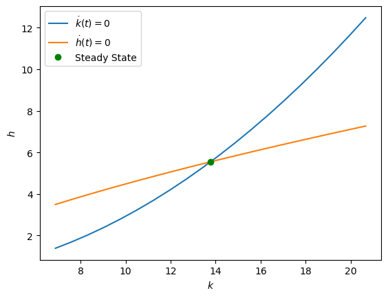
3. Organize our thinking by looking at special sets of points \((k,h)\) where at least one of the state variables happen to be at rest.

   • That is we seek to derive the \(k\)-nullcline,

     \[ N_k = \left\{(k,h) \in\mathbb{R}_{+}^{2} : T_{k}(k, h) = 0\right\}, \]

   • and the \(h\)-nullcline,

     \[ N_h = \left\{(k,h) \in\mathbb{R}_{+}^{2} : T_{h}(k, h) = 0\right\}. \]

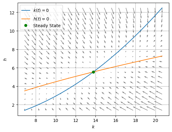
4. Using these sets as demarcation lines, and given the definition of the ODE map \(T\), deduce its induced vector field. The vector field tells us the ODE’s dynamic tendencies in the different quadrants separated by these two curves, \(N_k\) and \(N_h\).

   • Note that elements of the vector field along each of these nullclines, by definition, will be pointing in a direction that is perpendicular to the axis along which one of the state variables is at rest. (Think why this is so.)

   • Recall our ODE system:

     \[ \dot{\mathbf{x}}(t)= T\left(\mathbf{x}(t)\right). \]

     Or more verbosely,

     \[\begin{split} \left[ \begin{matrix} \frac{\text{d} k(t)}{\text{d}t} \\ \frac{\text{d} h(t)}{\text{d}t} \end{matrix} \right] = \left[ \begin{matrix} T_{k}(k(t), h(t)) \\ T_{h}(k(t), h(t)) \end{matrix} \right]. \end{split}\]

   • Take a current state in the phase space, i.e., in \((k, h)\)-space: This is the coordinate or point \(\left(k, h\right)\). At a fixed \(t\), the gradient vector induced by the ODE at the point \((k(t), h(t))\) is:

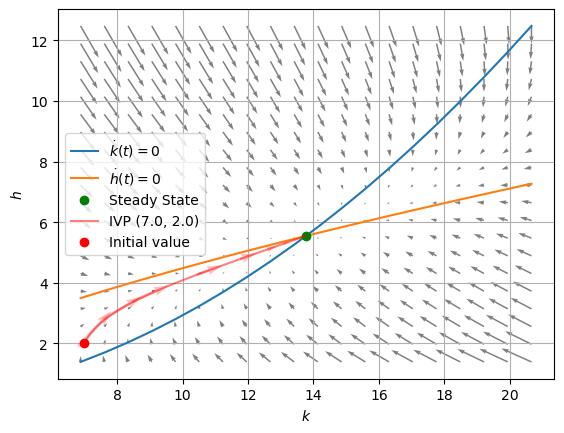
     \[ \frac{\text{d}h(t)}{\text{d}k(t)} = \frac{\frac{\text{d}h(t)}{\text{d}t}}{\frac{\text{d}k(t)}{\text{d}t}} = \frac{T_{h}(k(t), h(t))}{T_{k}(k(t), h(t))}. \]

     By definition the gradient vector would be a tangent to a solution curve that passes through that point!

   • Illustrate a particular solution curve in the phase space or \((k,h)\)-space beginning from a given initial value of the state variables.

Below, we plot a numerical example for the case where \(F\) is Cobb-Douglas.

Show code cell source Hide code cell source

import numpy as np
import matplotlib.pyplot as plt
from scipy.integrate import odeint

# Define model bits

def f(k, h, α, β):
    """Cobb-Douglas f"""
    return (k**β)*(h)**α

def T(state, t, s_k, s_h, n, g, δ_k, δ_h, α, β):
    """Equilibrium: ODE"""
    k, h = state
    kdot = s_k*f(k, h, α, β) - (n + g + δ_k)*k
    hdot = s_h*f(k, h, α, β) - (n + g + δ_h)*h
    return [kdot, hdot]

def T_zero(k, s_k, s_h, n, g, δ_k, δ_h, α, β):
    """Two sets of (k,h) pairs such that
    (1) dk/dt = 0, or
    (2) dh/dt = 0
    """
    # kdot = 0 locus
    h_kdotzero = ( s_k*k**(β-1.)/(n + g + δ_k) )**(-1./α)
    # hdot = 0 locus
    h_hdotzero = ( s_h*k**β/(n + g + δ_h) )**(1./(1.-α))
    return h_kdotzero, h_hdotzero
    
def steadystate(s_k, s_h, n, g, δ_k, δ_h, α, β):
    """Steady state equilibrium"""
    steady = lambda x, y, pow: ( (x**pow) * (y**(1. - pow)) )**(1./(1.-α-β))
    sk_drag = s_k/(n + g + δ_k)
    sh_drag = s_h/(n + g + δ_h)
    kss = steady(sh_drag, sk_drag, α)
    hss = steady(sk_drag, sh_drag, β)
    return kss, hss

# Parametric instance
s_k = 0.2
s_h = 0.1 
n = 0.001
g = 0.0017
δ_k = 0.08
δ_h = 0.10
α = 0.25
β = 0.5

# Solve for steady state
kss, hss = steadystate(s_k, s_h, n, g, δ_k, δ_h, α, β)

# Consider zooming into neighborhood around steady state
# Grids of k and h
N_grid = 20
kmin, kmax = 0.5*kss, 1.5*kss
# hmin, hmax = 0.5*hss, 1.5*hss
k_grid = np.linspace(kmin, kmax, N_grid)

# Nullclines are N_k ≡ (k_grid, h_kdotzero) and N_h ≡ (k_grid, h_hdotzero)
h_kdotzero, h_hdotzero = T_zero(k_grid, s_k, s_h, n, g, δ_k, δ_h, α, β)

def plot_nullclines(plt, k_grid, h_kzero, h_hzero, kss, hss):
    """Plot two sets of (k,h) pairs such that
    (1) dk/dt = 0, or
    (2) dh/dt = 0
    """
    plt.xlabel(r"$k$")
    plt.ylabel(r"$h$")
    plt.plot(k_grid, h_kzero, label=r"$\dot{k}(t)=0$")
    plt.plot(k_grid, h_hzero, label=r"$\dot{h}(t)=0$")
    plt.plot(kss, hss, 'og', label="Steady State")
    return plt

The nullclines are graphed below:

Show code cell source Hide code cell source

plt.figure()
plt = plot_nullclines(plt, k_grid, h_kdotzero, h_hdotzero, kss, hss)
plt.legend();

Next we show the vector fields induced by the ODE:

Show code cell source Hide code cell source

def phaseplot(plt, k_grid, h_grid, 
                        norm_grad=False):
    """Plot vector field"""
    X, Y = np.meshgrid(k_grid, h_grid)
    X = X.flatten()
    Y = Y.flatten()
    # Rates of change from ODE
    state = [X, Y]
    dx, dy = T(state, None, s_k, s_h, n, g, δ_k, δ_h, α, β)

    if norm_grad:
        # Normalize these vectors
        # Hide true magnitude
        norm = np.sqrt(dx**2. + dy**2.)
        U = dx / norm
        V = dy / norm
    else:
        # Un-normalized gradient vectors
        # Shows magnitude!
        U = dx 
        V = dy
        
    # Plot vector field
    plt.quiver(X, Y, U, V, angles='xy', alpha=0.5)
    # Grid lines for visual ease
    plt.grid()
    return plt

# Get the grid space for h to be of the same limit as that 
# implied by the plotted nullclines

# Lower bound of plot
hmin = min([h_kdotzero.min(), h_hdotzero.min()])

# Upper bound of plot
hmax = max([h_kdotzero.max(), h_hdotzero.max()])

# Grid of h
h_grid = np.linspace(hmin, hmax, N_grid)

plt.figure()
plt = plot_nullclines(plt, k_grid, h_kdotzero, h_hdotzero, kss, hss)
plt = phaseplot(plt, k_grid, h_grid,  
                        norm_grad=False)
plt.legend();

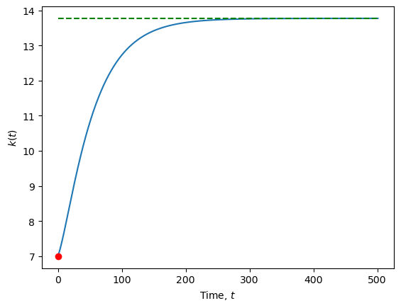
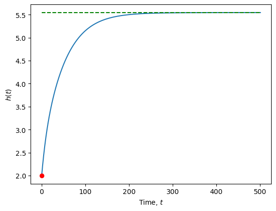
Below, we have the solution curve for the initial value problem beginning from a state \((k(0), h(0)) = (7,2)\):

Show code cell source Hide code cell source

# Time domain to perform integration
t_max = 501
mesh = 1001 # controls fineness of time interval
t = np.linspace(0., t_max, mesh) # grid approx of time domain

# Initial value of state
x0 = [7., 2.]

# Integrate ODE
psol = odeint(T, x0, t, 
              args=(s_k, s_h, n, g, δ_k, δ_h, α, β)
             )

# Sample a few points to show gradients
select_t = [10, 30, 50, 100, 150, 200, 250]
psol_t = psol[select_t, :]

# Show gradient on particular solution curve
ut, vt = T([psol_t[:,0], psol_t[:,1]], None, s_k, s_h, n, g, δ_k, δ_h, α, β)
norm = np.sqrt(ut**2. + vt**2.)

plt.figure()
plt = plot_nullclines(plt, k_grid, h_kdotzero, h_hdotzero, kss, hss)
plt = phaseplot(plt, k_grid, h_grid,  
                        norm_grad=False)
# Particular solution for IVP
plt.plot(psol[:,0], psol[:,1], '-r', alpha=0.5, 
            label="IVP ("+str(x0[0])+", "+str(x0[1])+")")
plt.quiver(psol_t[:,0], psol_t[:,1], 
           ut, vt, angles='xy', alpha=0.25, pivot="mid", 
                    width=0.0061, color="red")
plt.plot(x0[0], x0[1], 'or', label="Initial value")
plt.legend();

The particular solution is a function of time explicitly—i.e., \(t \mapsto (k,h)(t)\). Below we plot the trajectory of \(k\) and \(h\):

Show code cell source Hide code cell source

# Time path of solution, k(t)
plt.figure()
plt.plot(t, psol[:,0])
plt.plot(t[0], x0[0] ,'or')
plt.plot(t, kss*np.ones(t.shape), '--', color="green")
plt.xlabel(r"Time, $t$")
plt.ylabel(r"$k(t)$");

# Time path of solution, h(t)
plt.figure()
plt.plot(t, psol[:,1])
plt.plot(t[0], x0[1] ,'or')
plt.plot(t, hss*np.ones(t.shape), '--', color="green")
plt.xlabel(r"Time, $t$")
plt.ylabel(r"$h(t)$");

10.4. Cross-country income inequality

Cross-country income inequality

• What accounts for cross-country income inequality?

• Does the Solow-Swan insight on cross-country differences in long-run living standard hold in the face of other confounding factors?

Mankiw et al. [18] took the modified Solow-Swan model with human capital to cross-country data.

They showed that

1. the model accounts for cross-country differences in per capita income well; and,

2. allowing for human capital variation across countries and controlling for population growth and capital accumulation, there is conditional convergence. Convergence is at about the rate that the calibrated model predicts.

We’ll focus on their first contribution here.

10.4.1. Cross-cross version of the model

Suppose that each country \(j=1, \ldots, N\) has the aggregate production function:

\[ Y_j(t)=K_j^\beta(t) H_j^\alpha(t)\left(A_j(t) L_j(t)\right)^{1-\alpha-\beta}. \]

We get back the basic Solow model without human capital if we set \(\alpha=0\).

Anticipating variations in cross-country data, suppose in the model that countries differ in these features:

• saving rates in physical and human capital, respectively, \(s_{k, j}\) and \(s_{h, j}\);

• population growth rates, \(n_j\), and

• technology growth rates \(\dot{A}_j(t) / A_j(t)=g_j\).

Define \(k_j \equiv K_j / A_j L_j\) and \(h_j \equiv H_j / A_j L_j\).

There are a few more model-empirical assumptions to make:

• Each country \(j\) does not trade with another; and

• the data on per capita income for countries are roughly consistent with the countries being at or close to their respective steady state paths.

(One can’t possibly have a model of everything and test for anything under the sun!)

10.4.2. Balanced-growth living standard

The assumptions above allow us to derive the steady-state physical and human capital to effective labor ratios of country \(j,\left(k_j^*, h_j^*\right)\) as:

\[\begin{split} \begin{aligned} k_j^* & =\left[ \left( \frac{s_{k, j}}{n_j+g_j+\delta_k} \right)^{1-\alpha} \left( \frac{s_{h, j}}{n_j+g_j+\delta_h} \right)^\alpha \right]^{\frac{1}{1-\alpha-\beta}} \\ h_j^* & =\left[ \left( \frac{s_{k, j}}{n_j+g_j+\delta_k} \right)^\beta \left( \frac{s_{h, j}}{n_j+g_j+\delta_h} \right)^{1-\beta} \right]^{\frac{1}{1-\alpha-\beta}} \end{aligned}. \end{split}\]

Exercise 10.15

Show that the steady-state- or balance-growth-path income per capita of country \(j\) can be written as

\[\begin{split} \begin{aligned} \tilde{y}_j^*(t) & \equiv \frac{Y(t)}{L(t)} \\ & = A_j(t)\left( \frac{s_{k, j}}{n_j+g_j+\delta_k} \right)^{\frac{\beta}{1-\alpha-\beta}} \left( \frac{s_{h, j}}{n_j+g_j+\delta_h} \right)^{\frac{\alpha}{1-\alpha-\beta}} . \end{aligned} \end{split}\]

10.4.3. Balanced-growth and testable empirical model

Observe that if the \(g_j\)’s are not the same across countries, income per capita will diverge, since \(A_j(t)\), will be growing at heterogeneous rates.

Since technological progress is exogenous in the model, Mankiw et al. [18] assume a common rate of technical progress:

\[ A_j(t)=\bar{A}_j \exp (g t). \]

This assumption implies that although countries may have the same growth rate of technical progress, they can still differ in its level because \(\bar{A}_j\) can be heterogeneous.

Armed with this assumption, the balanced-growth-path of per-capita income (in logs) for each country \(j\) is:

\[ \ln \tilde{y}_j^*(t) = \ln \bar{A}_j+g t + \frac{\beta}{1-\alpha-\beta} \ln \left( \frac{s_{k, j}}{n_j+g+\delta_k} \right)+\frac{\alpha}{1-\alpha-\beta} \ln \left( \frac{s_{h, j}}{n_j+g+\delta_h} \right) . \]

Now we are getting close to a linear regression model that we can pass onto our empirical colleague (or self) to decorate with estimator party hats!

• If we can estimate \(\delta_k, \delta_h\) and \(g\) (from some other data sources), we can use cross-country data we can compute \(s_{k, j}, s_{h, j}, n_j\).

• Once we have these measures and since \(\ln \tilde{y}_j^*(t)\) is observable, this equation estimated by ordinary least squares (OLS) (i.e., by regressing income per capita on these measures) to get the estimates \(\hat{\alpha}\) and \(\hat{\beta}\).

Exercise 10.16 (Measurement issues)

How would one go about estimating \(\delta_k\) and \(\delta_h\)? (How did Mankiw et al. [18] do it?)

Empirically, most authors approximate \(s_{k, j}\) with average investment rates (i.e., the Investments-to-GDP ratio). Why?

Investment rates, average population growth rates \(n_j\), and log output per capita are available from the PWT.

Mankiw et al. [18] use the fraction of the school-age population that is enrolled in secondary school as a proxy for \(s_{h, j}\).

Note

Speed bump and a fork in the road

Despite the assumptions and empirical discipline, unfortunately we cannot rush out at this point to tell our STATA assistants to “just OLS it”.

Why?

The \(\ln \bar{A}_j\) term is unobserved to the econometrician. In the OLS regression, this will be subsumed under the regression error term. However, it is likely that \(\ln \bar{A}_j\)—and thus the regression error term—will be correlated with investment rates \(s_{k,j}\) and \(s_{h,j}\).

This gives rise to a problem of omitted-variable bias and this leads to inconsistent OLS estimates \(\hat{\alpha}\) and \(\hat{\beta}\).

At this juncture, we’ll have to make an additional assumption.[1]

Mankiw et al. [18] make the assumption that

\[ \bar{A}_j = A\varepsilon_{j} \]

and \(\varepsilon_{j}\) is orthogonal or uncorrelated with all other variables.

Now, the implied regression model can be estimated consistently:

\[\begin{split} \begin{aligned} \ln \tilde{y}_j^*= & \text { constant }+\frac{\beta}{1-\alpha-\beta} \ln \left(s_{k, j}\right)-\frac{\beta}{1-\alpha-\beta} \ln \left(n_j+g+\delta_k\right) \\ & +\frac{\alpha}{1-\alpha-\beta} \ln \left(s_{h, j}\right)-\frac{\alpha}{1-\alpha-\beta} \ln \left(n_j+g+\delta_h\right)+\varepsilon_j . \end{aligned} \end{split}\]

We reproduce the estimation result from Acemoglu [1]:

	MRW	Updated data
	1985	1985	2000
\(\ln \left(s_k\right)\)	.69	.65	.96
	\((.13)\)	\((.11)\)	\((.13)\)
\(\ln (n+g+\delta)\)	-1.73	-1.02	-1.06
	\((.41)\)	\((.45)\)	\((.33)\)
\(\ln \left(s_h\right)\)	.66	.47	.70
	\((.07)\)	\((.07)\)	\((.13)\)
Adj \(\mathrm{R}^2\)	.78	.65	.60
Implied \(\beta\)	.30	.31	.36
Implied \(\alpha\)	.28	.22	.26
Number of observations	98	98	107
Note: Standard errors in parentheses

The estimate of Adjusted \(R^2\) suggests that differences in cross-country physical and human capital investment behavior can account for about three quarters of income per capita differences.

This also implies that the original Solow [30] claim that differences in (black-box) TFP explain differences in cross-country living-standards can be somewhat overturned: That unexplained factor now only accounts for about a quarter of the cross-country income per capita differences.

This empirical insight of Mankiw et al. [18] led growth economists to focus on uncovering further how accumulation of physical and human capital may explain what was previously a “Solow-residual” TFP in order to explain economic growth with more economic structure—i.e., with endogenous growth theories.

10.5. Discussion

See the rest of Chapter 3 in Acemoglu [1].

Exercise 10.17

What other issues on measurement may arise in regard to the above empirical strategy?

How would you further relax the assumptions that Mankiw et al. [18] made, in order to further refine the empirical analysis?

---

[1]

Notice how doing empirical work is not just running a regression of something on anything, and pretending that this lets the data speak to us? It still comes with the cost of making modelling assumptions, whether we are prepared to be transparent about the model or have a loose idea of a model in our heads!