8. Qualitative Analyses#
Many nonlinear ODEs cannot be solved analytically.
However, in some settings we can still learn about the behavior of their solution without having to solve them.
That is, we can still learn about the dynamic behavior of a non-analytical ODE using a qualitative approach.
8.1. Phase diagram for scalar ODEs#
The tool we will use is graphical, and it is called a phase diagram.
Consider the equation
We can place \(\dot{x}\) on the vertical (or “\(y\)”) axis, and \(x\) on the horizontal (or “\(x\)”) axis.
If we know the shape or properties of \(g\) we can sketch its graph:
Given the shape (and other properties of) of \(g\), we can deduce the tendency or direction of the state, \(\dot{x}\), at each instance of the state variable \(x\).
Exercise 8.1
Consider the equation
We know that \(s, n \in (0,1)\), \(f(0)=0\), \(f'(x)>0\) for all \(x\), \(f'(x) \rightarrow 0\) as \(x \rightarrow \infty\) and \(f'(x) \rightarrow \infty\) as \(x \rightarrow 0\).
From this information, we can see that there are two forces acting on \(x\) determining how it will change at an instance: There is a positive force that contributes to \(x\) growing (i.e., \(\dot{x}>0\)) due to \(sf(x)\) being positive-valued in \(x\). However, the other force \(-nx\) acts in the opposition direction and creates a drag on growth in \(x\).
The question to ask is: At each possible instance of \(x\), what is \(\dot{x}\)?
Let’s use elementary curve sketching techniques to figure this out. Sketch the phase line:
Vector field: Draw a few example points of \(x\), and the corresponding vectors indicating the direction of instantaneous change, using what you know about \(\dot{x} = g(x)\). Explain your reasoning.
8.2. Phase diagram for two-variable ODEs#
Let’s have a look at some examples of phase plots for linear ODEs.
We can actually solve these ODEs analytically!
However, for the sake of understanding phase diagrams, let’s pretend we don’t know how to find these exact solutions.
Recall our purpose at this moment is to understand the solution qualitatively without having to explicit solve for it.
Show code cell source
# Import the relevant libraries to do this
import os
import numpy as np
import matplotlib.pyplot as plt
from control.phaseplot import phase_plot
from numpy import pi
8.2.1. Distinct real eigenvalues#
Recall from Section 7.1.2, when the eigenvalues of the linear ODE map, \(T(\mathbf{x}) = \mathbf{A}\mathbf{x}\), are distinct, the solution is characterized by a linear combination of straight-line solutions.
This in turn depends on the eigenvalues and their associate eigenvectors of the matrix \(\mathbf{A}\).
It turns out that the stability of a steady-state equilibrium of the system will depend on the signs of the eigenvalues.
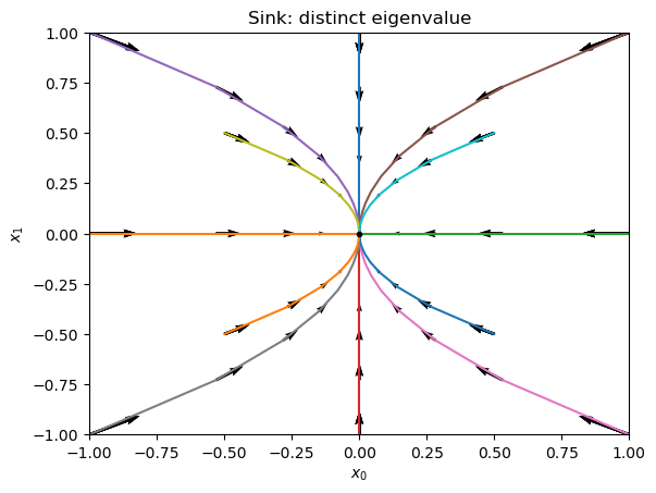
Case 1. Suppose \(\lambda_{1} < \lambda_{2} < 0\). Here’s an example where the system is de-coupled.
Example 8.1 (Another first-order ODE)
Consider the ODE:
where \(\mathbf{x} = (x_{0}, x_{1})\).
# Example, repeated positive root
λ_1, λ_2 = -0.6, -0.3

# Set up the linear map A
A = np.array([[λ_1, 0.0],
              [0.0, λ_2]])
Here’s the computer calculated version to verify these are the eigenvalues (and their associated eigenvectors):
Show code cell source
root, eigvec = np.linalg.eig(A)
print("The eigenvalues are")
print(root)
print("\nThe eigenvector(s) are (is)")
print(eigvec)
The eigenvalues are
[-0.6 -0.3]

The eigenvector(s) are (is)
[[1. 0.]
 [0. 1.]]
Vector field. Let’s discuss how we can deduce the dynamic behavior of the solution. To do this we figure out the vector field generated by the ODE.
The state space of the ODE here is the set of \((x_{0}, x_{1})\) coordinates in \(\mathbb{R}^{2}\). (Why?)
Use the ODE formula. Its right-hand side defines a vector field. The entire set of such slopes for all coordinates \((x_{0}, x_{1})\) is the vector field.
How would these two pieces of information inform us where the next state would be and therefore, where the “arrows” are pointing in the vector field?
Stream lines (solution curves). Recall Definition 4.1. Instead of visualizing the graph of the actual solution in \((\mathbf{x}(t), t)\) space—i.e., in \(\mathbb{R}^{k} \times \mathcal{T}\))—we can project it onto the state space itself. (This eliminates time explicitly from display in the solution curves.)
Continuing with the last example, we can plot a stream line (solution curve) beginning from a particular initial condition. This will describe the locus of \((x_{0}, x_{1})\) outcomes that satisfies the ODE, starting from a particular initial value.
In the figure below, we do this for several initial conditions stored. (In the code, these conditions are stored in the list X0.)
Exercise 8.2
Deduce analytically that the solution curves look like these:
Show code cell source
def distinctroots_ode(x, t):
    """ODE with repeated root vector field"""
    return A[0,0]*x[0] + A[0,1]*x[1], A[1,0]*x[0] + A[1,1]*x[1]

# Saddle
plt.figure()
plt.clf()
plt.axis([-1, 1, -1, 1])
# set(gca, 'DataAspectRatio', [1 1 1])
phase_plot(
    distinctroots_ode,
    scale=20,
    timepts=[0.05, 0.08, 0.1, 0.2, 0.5, 1.0, 1.5, 2., 3., 3.5, 10., 15.],
    X0=[
        [0, 1], [-1, 0], [1, 0], [0, -1],
        [-1, 1], [1, 1], [1, -1], [-1, -1],
        [-0.5, 0.5], [0.5, 0.5], [0.5, -0.5], [-0.5, -0.5],
    ],
    T=np.linspace(0, 20, 20)
)
plt.plot([0], [0], 'k.')
plt.xlabel('$x_0$')
plt.ylabel('$x_1$')
plt.title('Sink: distinct eigenvalue');
/home/obiwan/anaconda3/lib/python3.11/site-packages/control/phaseplot.py:985: FutureWarning: phase_plot is deprecated; use phase_plot_plot instead
  warnings.warn(
Exercise 8.3
Notice that the stream lines do not cross. Why?
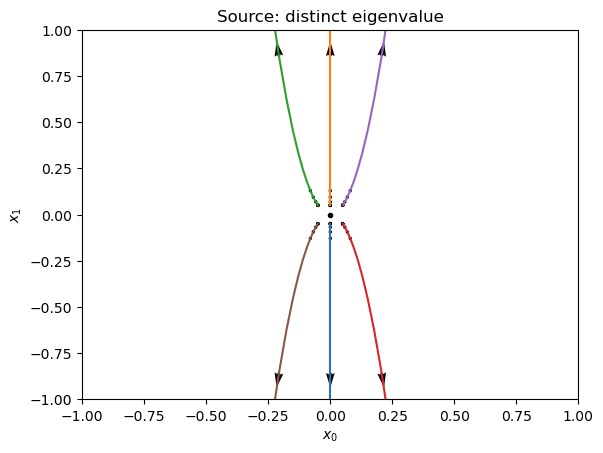
Case 2. Suppose \(0 < \lambda_{1} < \lambda_{2}\):
# Example, repeated positive root
λ_1, λ_2 = 0.3, 0.6

# Set up the linear map A
A = np.array([[λ_1, 0.0],
              [0.0, λ_2]])
Here’s the computer calculated version:
Show code cell source
root, eigvec = np.linalg.eig(A)
print("The eigenvalues are")
print(root)
print("\nThe eigenvector(s) are (is)")
print(eigvec)
The eigenvalues are
[0.3 0.6]

The eigenvector(s) are (is)
[[1. 0.]
 [0. 1.]]
Now the sample from the vector field and solution curves look like so:
Show code cell source
def distinctroots_ode(x, t):
    """ODE with repeated root vector field"""
    return A[0,0]*x[0] + A[0,1]*x[1], A[1,0]*x[0] + A[1,1]*x[1]

# Saddle
plt.figure()
plt.clf()
plt.axis([-1, 1, -1, 1])
# set(gca, 'DataAspectRatio', [1 1 1])
phase_plot(
    distinctroots_ode,
    scale=10,
    timepts=[0.05, 0.08, 0.1, 0.2, 0.5, 1.0, 1.5, 2., 5., 9.5],
    X0=[
        [0, -0.05], [0, 0.05],
        [-0.05, 0.05],
        [0.05, -0.05],
        [0.05, 0.05], [-0.05, -0.05],
    ],
    T=np.linspace(0, 10, 20)
)
plt.plot([0], [0], 'k.')
plt.xlabel('$x_0$')
plt.ylabel('$x_1$')
plt.title('Source: distinct eigenvalue');
Case 3 Suppose \(\lambda_{1} < 0 < \lambda_{2}\):
Example 8.2 (Another first-order ODE)
Consider the ODE:
where \(\mathbf{x} = (x_{0}, x_{1})\).
Exercise 8.4
Derive the eigenvalues and associated eigenvectors of \(\mathbf{A}\) by hand.
This is the phase plot with sample solution curves (or stream lines):
Show code cell source
def saddle_ode(x, t):
    """ODE with saddle point vector field"""
    return 1*x[0] - 3*x[1], -3*x[0] + 1*x[1]

# Saddle
plt.figure()
plt.clf()
plt.axis([-1, 1, -1, 1])
# set(gca, 'DataAspectRatio', [1 1 1])
phase_plot(
    saddle_ode,
    scale=2,
    timepts=[0.2, 0.5, 0.8],
    X0=[
        [-1, -1], [1, 1],
        [-1, -0.95], [-1, -0.9], [-1, -0.8], [-1, -0.6], [-1, -0.4], [-1, -0.2],
        [-0.95, -1], [-0.9, -1], [-0.8, -1], [-0.6, -1], [-0.4, -1], [-0.2, -1],
        [1, 0.95], [1, 0.9], [1, 0.8], [1, 0.6], [1, 0.4], [1, 0.2],
        [0.95, 1], [0.9, 1], [0.8, 1], [0.6, 1], [0.4, 1], [0.2, 1],
        [-0.5, -0.45], [-0.45, -0.5], [0.5, 0.45], [0.45, 0.5],
        [-0.04, 0.04], [0.04, -0.04]
    ],
    T=np.linspace(0, 2, 20)
)
plt.plot([0], [0], 'k.')
plt.xlabel('$x_0$')
plt.ylabel('$x_1$')
plt.title('Saddle point');
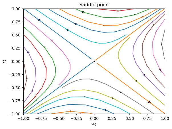
Exercise 8.5
Explain why the steady state equilibrium point here is called a saddle point?
(Use the ODE to deduce a few points in its induced vector field as seen in the figure above.)
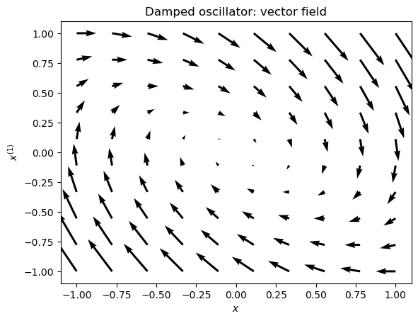
8.2.2. Complex eigenvalues#
Example 8.3
Consider the damped oscillator model earlier in Example 3.2.
We can deduce the qualitative dynamic behavior of the sytem by visualizing its phase diagram.
Recall this was a second-order ODE involving \(x(t)\) (position of the mass), \(\dot{x}(t)\) (its velocity), and, \(\ddot{x}(t)\) (its acceleration).
If we evaluate the formula defined by Equations (3.7) and (3.8) at a given coordinate \((x, x^{(1)})\), the left-hand side of (3.7) will tell us the rate of change of these two variables at the state \((x, x^{(1)})\).
Next we illustrate the vector field generated by Equation (3.7).
Show code cell source
def oscillator_ode(x, t, m=1.0, b=1.0, k=1.0):
    """Damped oscillator ODE. Returns velocity and
    acceleration at given state x and time t."""
    return x[1], -k/m*x[0] - b/m*x[1]

plt.figure()
# Sample grid points
Ngrid = 10
# Domains of x^(1) and x^(2)
S1 = [-1, 1, Ngrid]
S2 = S1
arrow_size = 0.15
phase_plot(oscillator_ode, S1, S2, arrow_size)
plt.xlabel('$x$')
plt.ylabel('$x^{(1)}$')
plt.title('Damped oscillator: vector field');
Exercise 8.6
Deduce that phase plots looks something like this below.
Show code cell source
# Generate a phase plot for the damped oscillator
plt.figure()
plt.axis([-1, 1, -1, 1])  # set(gca, 'DataAspectRatio', [1, 1, 1]);
phase_plot(
    oscillator_ode,
    X0=[
        [-1, 1], [-0.3, 1], [0, 1], [0.25, 1], [0.5, 1], [0.75, 1], [1, 1],
        [1, -1], [0.3, -1], [0, -1], [-0.25, -1], [-0.5, -1], [-0.75, -1], [-1, -1]
    ],
    T=np.linspace(0, 8, 80),
    timepts=[0.25, 0.8, 2, 3]
)
# Steady state point/equilibrium
plt.plot([0], [0], 'k.')
plt.xlabel('$x$')
plt.ylabel('$x^{(1)}$')
plt.title('Damped oscillator: vector field and stream lines');
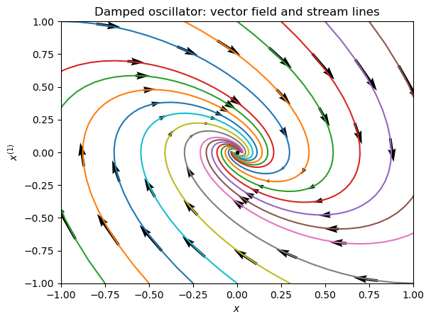
Exercise 8.7
Is the coordinate \((\bar{x}, \bar{x}^{(1)}) = (0,0)\) in the example above a (Lyapunov) stable, asymptotically stable, or unstable steady state equilibrium point?
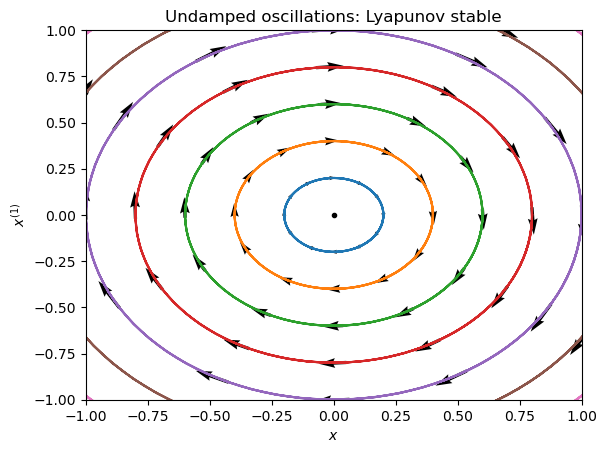
Example 8.4 (Undamped oscillations)
Consider Example 3.2 but now assume that there is zero damping force, or \(b=0\).
Here is the phase diagram with sample solution curves:
Show code cell source
# Stable
m = 1
b = 0 # no damping
k = 1
plt.figure()
plt.clf()
plt.axis([-1, 1, -1, 1])  # set(gca, 'DataAspectRatio', [1 1 1]);
phase_plot(
    oscillator_ode,
    timepts=[pi/6, pi/3, pi/2, 2*pi/3, 5*pi/6, pi, 7*pi/6,
             4*pi/3, 9*pi/6, 5*pi/3, 11*pi/6, 2*pi],
    X0=[[0.2, 0], [0.4, 0], [0.6, 0], [0.8, 0], [1, 0], [1.2, 0], [1.4, 0]],
    T=np.linspace(0, 20, 200),
    parms=(m, b, k)
)
plt.plot([0], [0], 'k.')
plt.xlabel('$x$')
plt.ylabel('$x^{(1)}$')
plt.title('Undamped oscillations: Lyapunov stable');
/home/obiwan/anaconda3/lib/python3.11/site-packages/control/phaseplot.py:1002: FutureWarning: keyword 'parms' is deprecated; use 'params'
  warnings.warn(
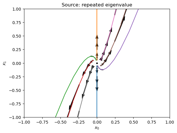
8.2.3. Repeated real eigenvalues#
Consider the two-variable (or second-order scalar) linear ODE where
The repeated eigenvalue is \(\lambda\).
Case 1. Suppose \(\lambda>0\):
# Example, repeated positive root
λ = 0.6

# Set up the linear map A
A = np.array([[λ, 0.0],
              [1.0, λ]])
Exercise 8.8
Compute by hand show that the eigenvalue is indeed repeated.
Here’s the computer calculated version:
Show code cell source
root, eigvec = np.linalg.eig(A)
print("The eigenvalues are")
print(root)
print("\nThe eigenvector(s) is (are)")
print(eigvec)
The eigenvalues are
[0.6 0.6]

The eigenvector(s) is (are)
[[ 0.00000000e+00  1.33226763e-16]
 [ 1.00000000e+00 -1.00000000e+00]]
Exercise 8.9
Deduce analytically that the solution curves look like these:
Show code cell source
def repeatedrootimproper_ode(x, t):
    """ODE with repeated root vector field"""
    return A[0,0]*x[0] + A[0,1]*x[1], A[1,0]*x[0] + A[1,1]*x[1]

# Saddle
plt.figure()
plt.clf()
plt.axis([-1, 1, -1, 1])
# set(gca, 'DataAspectRatio', [1 1 1])
phase_plot(
    repeatedrootimproper_ode,
    scale=10,
    timepts=[0.05, 0.08, 0.1, 0.2, 0.5, 1.0, 1.5, 2., 3., 3.5],
    X0=[
        [0, -0.05], [0, 0.05],
        [-0.01, 0.05], [-0.05, 0.05],
        [0.01, -0.05], [0.05, -0.05],
        [0.05, 0.05], [-0.05, -0.05],
    ],
    T=np.linspace(0, 10, 20)
)
plt.plot([0], [0], 'k.')
plt.xlabel('$x_0$')
plt.ylabel('$x_1$')
plt.title('Source: repeated eigenvalue');
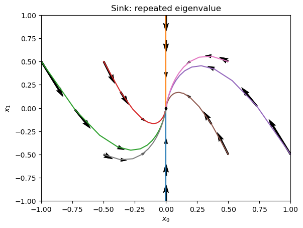
Case 2. Suppose \(\lambda<0\):
# Example, repeated positive root
λ = -0.6

# Set up the linear map A
A_neg = np.array([[λ, 0.0],
              [1.0, λ]])
Exercise 8.10
Compute by hand show that the eigenvalue is indeed repeated.
Here’s the computer calculated version:
Show code cell source
root, eigvec = np.linalg.eig(A_neg)
print("The eigenvalues are")
print(root)
print("\nThe eigenvector(s) are (is)")
print(eigvec)
The eigenvalues are
[-0.6 -0.6]

The eigenvector(s) are (is)
[[ 0.00000000e+00  1.33226763e-16]
 [ 1.00000000e+00 -1.00000000e+00]]
Exercise 8.11
Deduce analytically that the solution curves look like these:
Show code cell source
def repeatedrootsink_ode(x, t):
    """ODE with repeated root vector field"""
    return A_neg[0,0]*x[0] + A_neg[0,1]*x[1], A_neg[1,0]*x[0] + A_neg[1,1]*x[1]

# Saddle
plt.figure()
plt.clf()
plt.axis([-1, 1, -1, 1])
# set(gca, 'DataAspectRatio', [1 1 1])
phase_plot(
    repeatedrootsink_ode,
    scale=10,
    timepts=[0.2, 0.5, 0.8, 1.0, 1.8, 9.1],
    X0=[
        [0, -1], [0, 1],
        [-1, 0.5], [-0.5, 0.5],
        [1, -0.5], [0.5, -0.5],
        [0.5, 0.5], [-0.5, -0.5],
    ],
    T=np.linspace(0, 10, 20)
)
plt.plot([0], [0], 'k.')
plt.xlabel('$x_0$')
plt.ylabel('$x_1$')
plt.title('Sink: repeated eigenvalue');