7. A Quick Tutorial in Python Tools¶

A lot of models are quite sophisticated these days. Solving the models and evaluating the solutions are often non-analytic tasks. As a result, computational economics is a vital skillset for the modern economist to master. In this chapter, we will take a crash course on the basics of numerical computation in the Python language. While this is a very short and incomplete treatment on Python programming, fret not, as we will pick up more skills when we tackle specific problems. The best way to learn a language is while you’re fearlessly writing and speaking it!

7.1. Getting started¶

Go to the Anaconda distribution of Python and down the installer. (Choose the latest Python 3.xx version.)
Follow the instructions to install.
When you’re done you can start having fun with Python.

In this course, we will mostly use the Jupyter Notebook which allows you to write notes and do live computing within the notebook itself. I found this to be a great tool, not only for learning, but also for communicating works in progress with my research collaborators.

Jupyter should be installed with your Anaconda distribution. If not install it:

conda install jupyter

Sometimes, for longer codes, you may want to write your code as Python scripts or functions (and save them in the format, mysourcecode.py).

You can create and edit your Python code using any editor you like. My current favorite is Atom. This is a free editor.

Then you can run the code as a batch of instructions. A nice interactive Python interface is called IPython. This comes with your Anaconda distribution. Launch IPython at your terminal (or click on its icon if you’re a Windows user):

ipython

You should see a window like this popping up:

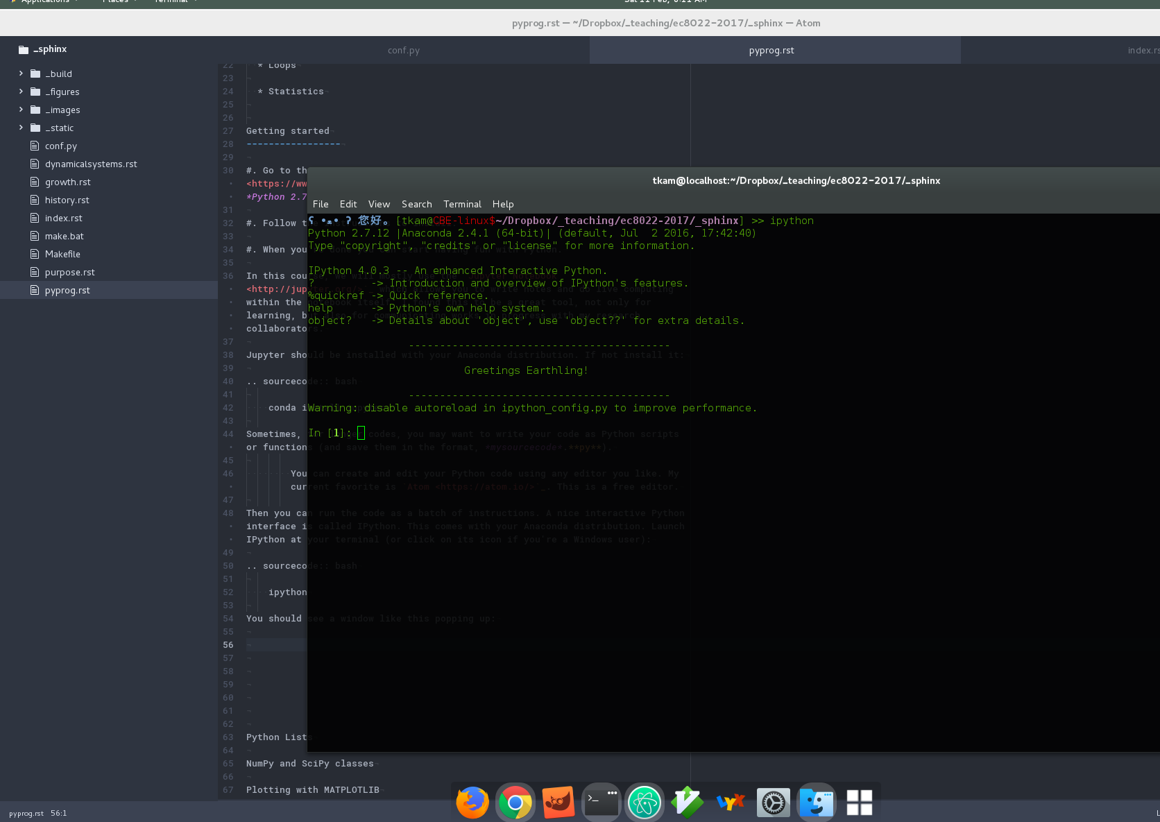
An Ipython terminal with Atom editor lurking behind

We will walk through Ipython and Jupyter Notebooks soon when we get to the live TutoLabo sessions with my assistant Igor.

Python is an interpreted language. This means you write code that is very close to human language, and its interpreter converts that to machine-level code that your computer can operate on.

Some of you may have had experience with other scientific programming languages like R, MATLAB, Julia and etc. Well, Python is just like that. But in my opinion, Python’s language is highly readable.

7.2. Data Types¶

In your modelling work you will often be dealing with different data types for variables. Typically, these are

Floating-point numbers or “floats”
Integers
Boolean
strings

We’ll work through these by example.

7.2.1. Floats¶

Since a computer can only store discrete information, a continuous object like a real number can only be represented approximately.

The recent film Hidden Figures was a true story about black women working as “colored” computers and engineers for NASA in the 1950-60s. Back in the day, a computer was a human doing intensive calculations by hand. At the time, much of the calculations in solving numerical differential equations were done by hand with the aid of log tables. Later, when they began to replace human computers with IBM machines, there was a scene where the human computer detected huge errors in the machine computer’s calculations of a space capsule trajectory. This was due to the limited precision of early machine computers. The human computer was also limited in precision!

(The film also highlighted the ugly face of institutionalized racism , sexism, and white privilege.)

\(\bigstar \bigstar \bigstar \bigstar\)

A floating point number is a computer’s approximation of a real number, e.g., \(\pi\), to some finite precision. Check this out in your Ipython terminal:

In [1]: import numpy as sweetpotato
In [2]: print(sweetpotato.pi)
3.14159265359

In Python you have to be pedantic when you intend to use floats. For example:

In [3]: x= 3.0

In [4]: type(x)
Out[4]: float

Notice the explicit use of a decimal or period after a number. This make the variable x a floating point representation of a real number.

7.2.2. Integers¶

From the previous example, supposed we had accidentally typed

In [7]: x= 3

In [8]: type(x)
Out[8]: int

Notice the lack of a decimal or period after a number. This make the variable x an integer now. We will quite often use integers for indexing elements in a Python list, or, a Numpy array.

7.2.3. Boolean¶

The Boolean data type can have values True or False. For example:

In [10]: x, y, z = True, False, True

In [11]: print(x,y,z)
(True, False, True)

In [12]: x+y
Out[13]: 1

In [14]: x+z
Out[14]: 2

Observe that we can do Boolean algebra with these data types.

7.2.4. Strings¶

Example:

In [16]: x = "Hello Dave"

In [17]: print(x)
Hello Dave

7.3. Python Lists, Indexing and Slicing¶

A Python list is a collection of Python objects. For example

In [16]: mylist = [ "Hello Dave", 2.0, 3.4 ]

In [17]: mylist[0]
Out[17]: 'Hello Dave'

The last instruction is an example of indexing, where we picked out the first element of mylist which is indexed by the integer 0.

Note

Python indexes begin from the integer 0.

Here’s a quick way to get the last element of that list:

In [18]: mylist[-1]
Out[18]: 3.4

We can also do slicing, i.e., extract chunks of data we want from a Python list. Here’s an application of this idea to the previous example’s mylist.

In [19]: mylist[0:2]
Out[19]: ['Hello Dave', 2.0]

This example picked out the first and second elements of mylist.

Here’s the syntax for slicing in general on a Python list a:

a[start:end] # members from arbitrary START to END-1
a[start:]    # members from arbitrary START through the rest of the array
a[:end]      # items from the beginning of list through END-1
a[:]         # a copy of the whole array

Note

Commenting your code lines. Notice the # symbols above followed by text comments? The # decoration makes the stuff that come after it invisible to Python’s interpreter and can only be read by the human.

Writing comments after or around your lines of code is a good programming practice. Can you imagine why? (Think about revising your code 6 years after you’ve first developed your code!)

We can also have a python list of lists, so on and so forth:

In [19]: mylist = [ "Hello Dave", 2.0, 3.4, [1,2,3,4] ]

In [20]: mylist[3]
Out[20]: [1, 2, 3, 4]

Python lists come overloaded with additional functions, like:

In [21]: mylist.pop(3)
Out[22]: [1, 2, 3, 4]

where mylist.pop(3) removes the last element of mylist. Alternatively, if you wanted to pop out the last element of a list, you could also have written mylist.pop(3). Either way, we can now check what happened to the original list called mylist:

In [23]: print(mylist)
Out[24]: ['Hello Dave', 2.0, 3.4]

We can also do the reverse:

In [25]: mylist.append(["This is fake news"])

In [26]: mylist
Out[27]: ['Hello Dave', 2.0, 3.4, 'This is fake news']

7.4. Python dictionaries¶

Another useful thing is an object called a Python dictionary. This will come in handy when you are generating heaps of data and you want to label them and extract them later, without having to keep track of thousands of variables or objects as inputs or outputs to functions. To store these things neatly as a single object, you can use a Python dictionary.

Note

Think about your kitchen drawer: Are you the sort of cook who compartmentalizes your knives from forks, your ladles from your spatulas? If that’s you, then creating a Python dictionary works the same way: It helps you organize things better.

Here’s a simple example of a dictionary that maps keys to values

In [10]: d = dict(alice=0.1, bob=[1,2,3], christine='Is Not Alice or Bob')

In [11]: d['christine']
Out[11]: 'Is Not Alice or Bob'

In [12]: d['alice']
Out[12]: 0.1

Another equivalent way to create the previous example is

d = {'alice': 0.1, 'bob': [1, 2, 3], 'christine': 'Is Not Alice or Bob'}

7.5. NumPy and SciPy libraries¶

Two of the most used libraries for scientific computing are NumPy and SciPy. In this course, we will use predominantly tools contained in Numpy.

7.5.1. NumPy Lists, Indexing and Slicing¶

From a Python list we can convert it into a Numpy array:

In [39]: import numpy as np

In [40]: y = np.asarray(mylist)

In [42]: print(y)
['Hello Dave' '2.0' '3.4' 'This is fake news']

In [43]: type(y)
Out[43]: numpy.ndarray

We can convert it back to a Python list when required:

In [44]: z = y.tolist()

In [45]: type(z)
Out[45]: list

We will work with NumPy arrays a lot in our numerical computations later.

Note

Have a tour of NumPy’s tutorial here and also this here for SciPy. We will use SciPy later for tasks like solving optimization problems, and, function approximation.

Here’s an example for creating a two-dimensional matrix or NumPy array:

In [17]: A = np.array([[1, 2, 3], [4, 5, 6]])

In [18]: A
Out[18]:
array([[1, 2, 3],
       [4, 5, 6]])

In [19]: A.size
Out[19]: 6

In [20]: A.shape
Out[20]: (2, 3)

In the above example, what we’ve done is stack two \(1 \times 3\) row vectors vertically in a list, and using the NumPy class’ function called array(), we turn the list into a NumPy matrix. The last two command inputs, respectively, check the number of elements in the matrix A and the dimension of that matrix.

The reason we will often work with NumPy arrays is that in NumPy and SciPy, we can avoid writing loops to speed things up. NumPy arrays come overloaded with many useful functions that can be used to perform quick operations on an array itself. To see what these functions are, take the A matrix created earlier. Now, type a period after A, and hit the “Tab” key on your keyboard:

In [23]: A.
A.T             A.argsort       A.compress      A.cumsum        A.dumps         A.imag          A.min           A.prod          A.reshape       A.shape         A.sum           A.tostring
A.all           A.astype        A.conj          A.data          A.fill          A.item          A.nbytes        A.ptp           A.resize        A.size          A.swapaxes      A.trace
A.any           A.base          A.conjugate     A.diagonal      A.flags         A.itemset       A.ndim          A.put           A.round         A.sort          A.take          A.transpose
A.argmax        A.byteswap      A.copy          A.dot           A.flat          A.itemsize      A.newbyteorder  A.ravel         A.searchsorted  A.squeeze       A.tobytes       A.var
A.argmin        A.choose        A.ctypes        A.dtype         A.flatten       A.max           A.nonzero       A.real          A.setfield      A.std           A.tofile        A.view
A.argpartition  A.clip          A.cumprod       A.dump          A.getfield      A.mean          A.partition     A.repeat        A.setflags      A.strides       A.tolist

Note the tolist() function that we’ve already discussed above. Here’s a few useful ones for our purposes. The ravel() function basically gives a flattened view of the array A without actually flattening or vectorizing it; so no new memory real estate is being consumed here:

In [23]: A.ravel()
Out[23]: array([1, 2, 3, 4, 5, 6])

In contrast the flatten() command flattens or vectorizes the array A and requires new memory space:

In [23]: a = A.flatten()

In [27]: a
Out[27]: array([1, 2, 3, 4, 5, 6])

This is equivalent to doing:

In [29]: A.reshape(1,-1)
Out[29]: array([[1, 2, 3, 4, 5, 6]])

What this example does is to reshape the \(2 \times 3\) array A into a row vector. (The argument 1 forces the row, and the second argument -1 says automatically fit everything else in.)

7.6. Plotting with MATPLOTLIB¶

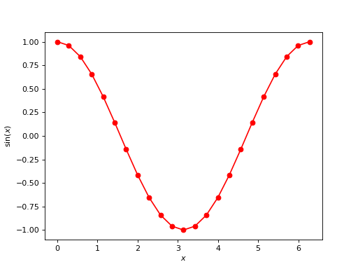
Let’s start with plotting a 2D graph:

Construct a uniformly-spaced grid of 23 elements, ranging from \(0\) to \(2\pi\). This will be the domain of our function. In the code, we store them as the NumPy array x.
Plot the graph of a cosine function evaluated at these points. This will be stored in memory as the array y.
Don’t forget to label your axes!

Here we go:

import matplotlib.pyplot as plt
import numpy as np
plt.figure()
x = np.linspace(0.0, 2.0*np.pi, 23)
y = np.cos(x)
plt.plot(x,y, 'o-r')
plt.xlabel('$x$')
plt.ylabel('$\sin(x)$')
plt.show()

(Source code, png, hires.png, pdf)

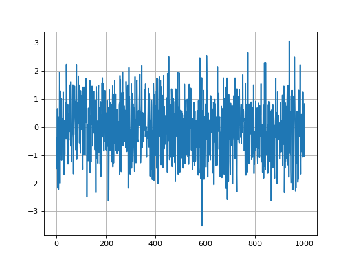
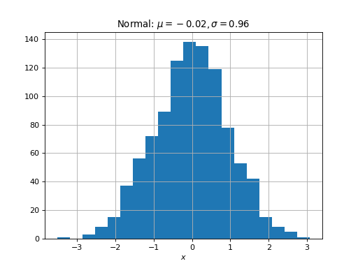
In the next example, we use NumPy to generate a sequence realizations of a Gaussian random variable and then we plot two figures:

The sample path.
A histogram to illustrate the sample distribution.

import matplotlib.pyplot as plt
import numpy as np

# Random Gaussian data
x = np.random.randn(1000)

# First figure-sample sequence
plt.figure()
plt.plot(x)
plt.grid()

# Second figure-histogram of sample
plt.figure()
plt.hist( x, 20)
plt.grid()
plt.xlabel('$x$')
plt.title(r'Normal: $\mu=%.2f, \sigma=%.2f$'%(x.mean(), x.std()))

plt.show()

(Source code)

(png, hires.png, pdf)

(png, hires.png, pdf)

This example illustrates the use of the plt.figure() function to create a new figure without writing over an existing figure. This is useful in a script context when you are generally multiple plot at the same time.

There are lots of additional examples in the MATPLOTLIB website gallery. You can learn from these and adapt them to your own applications later.

7.7. Useful Python and Numpy functions¶

To create a list of integers counting from \(0\) to \(N-1\):

In [1]: N=5

In [2]: range(N)
Out[2]: [0, 1, 2, 3, 4]

This is often useful when we do repeated evaluations using loop statements. See below.

7.8. Conditionals¶

Think about writing down a state contingent decision rule for your robot butler. For example: If the temperature is 18.1 degrees celcius or less, then turn on the heater. If the temperature is 29 degrees celcious or more, then turn on the cooling system. Otherwise, do nothing.

Similar, in talking to Python to execute your commands, quite often your commands will be state contingent. Here an example:

# import NumPy library
import numpy as np

# Generate realization of uniform random variable on [0,1]
x = np.random.rand(1)

# Test x condition:
if x < 0.2:
  print("Jump to your left. x = %0.3f" % (x))
else:
  print("Jump to your right. x= %0.3f" % (x))

Try this out in your IPython console. See what you get.

Sometimes you may need to issue compound conditional statements. Doing this in Python is quite natural in terms of syntax.

Note

Just be careful of two things:

Indents: Python uses indentations for statements that are nested within conditions.

Colons: after the conditions following IF, ELIF or ELSE statements.

Let’s see these is an example:

x = 0.214567
test = "apple"
if x <= 0.2 and test != "apple":
  print("Yolo!")
elif x >= 0.2 and test == "apple":
  print("Pine"+test+"pen")
else:
  print("Some of the complementary conditions hold")

Can you try deciphering what this says?

7.9. Loops¶

Python also comes with a useful function called enumerate(). This allows you to extract two arguments: First, the integer index for each element of the list we pass to enumerate(). Second, the element itself associated with the first argument. To fix ideas, let’s look at this example:

# Create NumPy array of 15 evenly spaced numbers from .1 to 2.
x = np.linspace(0.1, 2.0, 15)

# Loop over this array and print each element out
for i in range(x.size):
  print(x[i])

The range() function creates a list of integer indexes for each element of the array x, which should count from 0 to 14, in this example.

A FOR loop is useful, as in the example above, when you know exactly when the loop will finish its iterations.

You should get:

1
235714285714
371428571429
507142857143
642857142857
778571428571
914285714286
05
18571428571
32142857143
45714285714
59285714286
72857142857
86428571429
0

A cooler way to do this is

for i, x_i in enumerate(x):
  print("%i \t %0.5f" % (i, x_i))

You should get this output:

The enumerate() function gives you two things at once in a loop: the index or counter of the element of an array or list, and, the element itself. Note the fancy arguments in the usage of the print() command above? Can you decipher it?

Note

Just be careful of two things:

Indents: Python uses indentations for statements that are nested within FOR or WHILE loops.

Colons: after the conditions following FOR or WHILE statements.

Depending on your application, sometimes you might want to use a WHILE loop instead of a FOR loop. (Usually, this would be the case when you don’t know when the loop will terminate.)

Here’s an example with a convergent sequence of real numbers generated by the formula:

\[y = \frac{1}{5 \left( 1 + x \right)}, \qquad x \geq 0\]

# Tolerance for zero
TOL = 1e-3
# Arbitrary initialization
x, y = 0.0, 1.0
# The while loop
while y > TOL:
    d = 1.0 + x
    y = 0.2/d
    x = d
    print("\ny = %0.5f" %(y))

which outputs:

y = 0.2000

y = 0.1000

y = 0.0667

y = 0.0500

y = 0.0400

y = 0.0333

y = 0.0286

y = 0.0250

y = 0.0222

y = 0.0200

y = 0.0182

...

y = 0.0011

y = 0.0010

7.10. Statistics¶

Have a browse through this tutorial here at SciPy Tutorials

7.11. More Python resources for the economist¶

Since this is a course about macroeconomic modelling, not a course on Python programming, we will be introducing Python and its various usages on the fly. This chapter gave you some essential tools, by example. The only way you will begin to think and speak Python in your economic modelling and application, is to force yourself to put it into action: Code from scratch, don’t be afraid to get stuck, and keep trying. We will supply you with basic model templates in Python, but you should not just take a code or library of codes as it is. Take it apart and try re-writing your own version line by line. (Take a peek at our given examples if you like, but try to think by yourself too.) You will appreciate the hard work at the end.

If you want to spend time learning NumPy and SciPy systematically, a great place to do this is at the Scipy Lectures.

The QuantEcon project is a great source to learn Python in the context of economic modelling, or vice-versa. I highly recommend it. It also comes with the same tutorials in the up and coming language Julia.

Don’t worry if you don’t remember every command or syntax when you use Python, NumPy or SciPy. You can always Google it! (I still do.) Here is a useful cheat sheet for commonly used commands for scientific computing.

For those coming over from the dark side of proprietary software like MATLAB to Python/NumPy/SciPy, check this cheat sheet out.

Finally, learning the syntax of a language is one thing. Actually being able to use the language in your work successfully comes with trying and getting your own hands dirty.

Warning

Keep in mind: If you don’t have a good understanding of the theory behind a problem you’re trying to compute, and, if you don’t think creatively in your solutions approach, then having an elephant’s memory of the language’s syntax will not get you very far.