2. A Brief History

Key Learning Points

• Historical foundations of Macroeconomics
• Lucas Critique:
  • Economic equilibrium as statistical model
  • But statistical model may not be an equilibrium

Some say the field of Macroeconomics began with John Maynard Keynes’ 1936 magnum opus, The General Theory of Employment, Interest and Money. Keynes had catalyzed a metaphysical split between the study of individuals and firms at the microeconomic level (i.e., microeconomics or price theory) from the study of an economy as a whole, and its systemic relation to aggregate government policy.

Keynes’ verbal narrative alluded to the idea of the economy as a mechanical, dynamical system consisting of interacting sectors of the economy (e.g., consumption, investment, government). Elsewhere in Eastern Europe, a similar idea was in place (Michal Kalecki). But since Kalecki wrote in Polish, nobody in the English-speaking world paid attention! [Ka1935] had also applied the field of mathematical dynamics to think about the Business Cycle (or Trade Cycle as people were wont to call it in the old days).

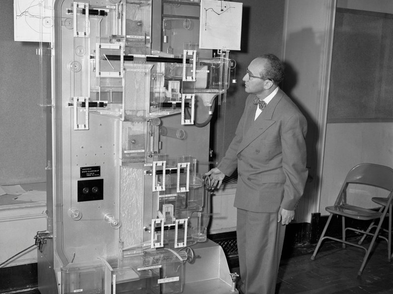
The MONIAC IS/LM model Source: Smithsonian Magazine [Fe2014]

The early formalization of Keynes’ idea took the form of the famous IS/LM model. This stuff is taught in elementary undergraduate macroeconomics courses today, albeit in modified forms as the IS-LM-MP or AD-AS model. This modelling device was invented by Sir John R. Hicks, in [Hi1937]. While it was an instructive mathematical device, it was a static one. As a consequence, one could not explicitly analyze dynamic phenomena like the evolution of capital, equity, government debt and so on. From Hick’s toy IS/LM representation, Jan Tinbergen and others (e.g., Lawrence Klein and Arthur Goldberger) grew larger econometric beasts from the original Keynes-Hicks macroeconomic paradigm [HH1989]. These models were used in many countries for macroeconomic forecasting and counterfactual policy experiments. A crucial feature of these macroeconometric models was that they did not require specifications of economic decision making at the level of agents: households and firms. This allowed for unrestricted parametrization of the model structure. In a way, this gave a lot of flexibility to the econometrician, since one could parametrize the model freely (e.g., by adding arbitrary causal channels and dependency on lagged information) in order to fit historical data.

On another spectrum—and in fact, chronologically preceding the works of Kalecki, Keynes and Hicks—the mathematician Frank Ramsey had solved an important problem on optimal saving in 1928: see [Ra1928].

This was a dynamic optimal decision-making problem. Its solution was an optimal savings function, as a function of time. Central to the characterization of this solution was a mathematical object called the Euler-Lagrange functional equation. (This was a differential equation.) Thus, being able to solve this equation meant one was able to figure out the “best” path a decision maker in the model should take over time.

Ramsey’s contribution to Economics would not impact on the practice of modern macroeconomics until the 1960’s when people like David Cass, Tjalling Koopmans, Kenneth Arrow and Mordecai Kurz paid attention to Ramsey’s pathbreaking application of the calculus of variations in his 1928 paper.

Much of modern macroeconomic theory is still based on similar functional analytic problems. However, our modern problems will be generalized to much more sophisticated settings (e.g., with many actors making dynamic decisions) and economically more difficult questions (e.g., how to characterize optimal government policy in the face of dynamic informational and incentive constraints; and how to solve a dynamic economy when the notion of a state variable includes an infinite-dimensional object, a distribution over agents with heterogeneous attributes).

You might ask: Why are there so many different macroeconomic models? How are they different? First, horses for courses: It is an extremely difficult task to have a single model of everything; it will be just too complex to understand what’s going on in the model.

Try building a map of your city with every detail in it: from every blade of grass to every dog peeing on a tree. See how useful such a map of your world will be!

Second, what can vary, from one model to another, will be part of the economists storyboard:

• the set of actors (private and public agents),
• agent preference sets (and their functional representations),
• assumptions about information (including sources of uncertainty),
• commodity spaces (and production sets),
• market pricing mechanisms (e.g., perfect competition, monopoly, bilateral bargaining).

By the 1970s, economists were concerned with the failure of macroeconomic policy in alleviating recessions during the Oil Crises. The more governments tried using fiscal and monetary policy to stabilize aggregate demand, the more recessionary their economies became. Some economists began looking to a new bechmark paradigm where aggregate economic outcomes were consistent with one’s story of microeconomic behavior and the micro-agent’s expectations of future events (including government policy plans). This led to the so-called rational expectations revolution.

The notion of rational expectations was not meant to be taken to be a definitive concept of how people formed beliefs about future policies and events. It was nevertheless a useful equilibrium concept for a modeller to capture the idea that an an estimated “reduced-form” econometric model (along the lines of Tinbergen’s early work) may not be stable in the face of policy changes. You see, up until then, policy analysts were doing conterfactual policy experiments on their estimated Keynesian macroeconometric models, while presuming that the structure of their models (i.e., magnitude and direction of causal relations) were invariant to their policy experiments. In short, they treated the economy and market participants like a physical engineering system where the underlying atoms are not sentient (i.e., they do not think or make decisions).

However, in a sentient economy, agents can look ahead and form beliefs about future events, including policy changes. This means that they can form best responses to anticipated policy changes. The resulting equilibrium representation—i.e., the statistical law or mathematical counterpart to Keynesian macroeconometric structures—may actually shift, in both magnitude and direction when policies change. That is, the statistical process for the economy may not be policy invariant. For example, up until then, economist presumed that there was a stable statistical inflation-unemployment trade-off given by the Phillips curve. This statistical relationship formed the basis for most Keynesian models’ monetary policy trade-off: Policy makers decide on a particular policy outcome and locate the economy as a point on that trade-off curve. However, [Lu1972] gave an example of the Phillips curve inverting, when agents anticipate prolonged government intervention in monetary policy, thus nullifying the effectiveness of the policy. (See also [Lu1976].)

Thus, the so-called Lucas Critique and its related rational expectations equilibrium concept, was not so much a push to indoctrinate economists and the general public with some right-wight economic policy agenda, as many popular writers mistakenly label it. Lucas’ point was to provide a counter-example showing the perils of policymaking based on mechanical/statistical models of the economy; i.e., econometric models that do not build in the contingency of sentient, forward-looking and optimally reactive agents (i.e., “the markets” in popular parlance), in the face of policy change.

In contrast to the Old Keynesian macroeconometric modelling philosophy, the modern microfoundation approach now places a lot of logical discipline, or restrictions on (equilibrium-determined) parameters of the resulting probability model vis-a-vis observed data. While a benefit in terms of delivering consistency in narratives in terms of internal model logic, these models made the life of the econometrician very difficult. (Can you think why?) As a consequence, for a few decades, there had been a marked bifurcation in research paths between macroeconomic modellers and time-series macroeconometricians. However, we now live in exciting times: With recent technological advancements in computing and also in econometric theory, researchers have again found new interest in estimating and testing microfounded macro models with data.

In this course, we will learn about some of these modern approaches to macroeconomics, by example. As a consequence, we will learn to tame different horses for different courses. We close this chapter with two questions: So why is the practice of macroeconomics so controversial? Does that not make the field exciting to study and to work in?

[Fe2014]

Fessenden, M. This Computer From 1949 Runs on Water. Link

[Hi1937]

Hicks, J. (1937). Mr. Keynes and the “Classics”; A Suggested Interpretation. Econometrica, 5(2), 147-159. https://www.jstor.org/stable/1907242

[HH1989]

Hughes Hallett, A. J. (1989). Econometrics and the Theory of Economic Policy: The Tinbergen-Theil Contributions 40 Years On. Oxford Economic Papers, 41(1), new series, 189-214. http://www.jstor.org/stable/2663189

[Ka1935]

Kalecki, M. (1935). A Macrodynamic Theory of Business Cycles. Econometrica, 3(3), 327-344. https://www.jstor.org/stable/1905325

[Lu1972]

Lucas, R. (1972). Expectations and the neutrality of money, Journal of Economic Theory, 4(2), 103-124. http://dx.doi.org/10.1016/0022-0531(72)90142-1

[Lu1976]

Lucas, R. (1976). “Econometric Policy Evaluation: A Critique”. In Brunner, K.; Meltzer, A. The Phillips Curve and Labor Markets. Carnegie-Rochester Conference Series on Public Policy. 1. New York: American Elsevier. pp. 19–46

[Ra1928]

Ramsey, F. (1928). A Mathematical Theory of Saving. The Economic Journal, 38(152), 543-559. https://www.jstor.org/stable/2224098