5. State Space Computations¶

Now we describe the implementation for the key tasks involved so far. We will need to:

compute state state partitions: $D := \cup_{k=1}^{K}Q_k$ ;
construct transitions from each subspace $Q_k$ into corresponding sets $P(a)(Q_k) \subset D$ , for every possible action profile $a \in A$ ;
record intersections $P(a)(Q_k) \cap Q_k'$ , for every $k,k' \in \mathbf{K}$ ; and
sample uniform points from each $Q_k$ , and check for nonempty samples that end up transitioning to each respective intersecting set $P(a)(Q_k) \cap Q_k'$ .

5.1. Storage¶

We only need to store:

each index $k' \in \mathbf{I}(a,k) \subseteq \mathbf{K}$ , which refers to some partition element(s) $Q_{k'}$ whose subset $Poly_{k'}$ is accessible from $Q_{k}$ given operator $P(a)$ .
- This suffices for indexing the correct slices of equilibrium payoff sets over the corresponding subset $Poly_{k'}$ of the state space $D$ .
the finite number of vertices of each $Poly_{k'}$ and the corresponding linear (weak) inequality representation of each $Poly_{k'}$ .
- This will become apparent later when we solve separable bilinear programming problems where it involves optimizing over these subsets $Poly_{k'}$ (when constructing max-min punishment values in the game).
the sub-samples from all the Hit-and-Run realizations that belong to every partition element $Q_k$ which will end up in particular intersections summarized by each polytope $Poly_{k'}$ .

5.2. Implementation¶

Since we have finite partition elements $Q_{k}$ and finite action profile set $A \ni a$ , then we can enumerate and store all intersections previously denoted by $\{ Poly_{k'(k,a)}: \forall a \in A, k \in \mathbf{K} \}$ or equivalently by their index sets $\{ \mathbf{I}(a,k): (a,k) \in A \times \mathbf{K} \}$ .

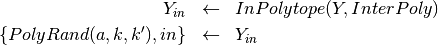
Pseudocode

For each $(a,k)\in A \times \mathbf{K}$ :

Get vertex representation of $Q_k \in D$
Set $P(a)$ as $P$
Get vertex representation $T$ from $P(Q_k)$
Simulate Hit-and-Run uniform realizations in simplex $T$ . Get

$X := \{ \lambda_n \}_{n=1}^{N_{sim}} \leftarrow RandomPolyFill(N_{sim},T)$
Set $i \leftarrow 0$
For each $k' \in \mathbf{K}$ :
- Get vertex representation of $Q_k' \in D$
- Get intersection $InterPoly = Q_{k'} \cap T$ (a polytope) as:
$InterPoly \leftarrow PolyBool(Q_{k'},T)$
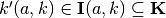
- If $InterPoly \neq \emptyset$ :
  Set $i \leftarrow i + 1$
  
  Store index to partition elements $Q_{k'}$ when $InterPoly$ is nonempty. Set
  
  $TriIndex(a,k)(i) \gets k'$
  
  Store vertex data of polytope. Set:
  
  $PolyVerts(a,k,k') \gets Interpoly$
  
  Store linear inequality representation of the same polytope. Set:
  
  $PolyLcons(a,k,k') \gets Vert2Lcon(InterPoly)$
  
  Map Monte Carlo realizations $X$ under operator $P$ . Set:
  
  $Y \gets P(X)$
  
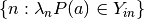
  List members of $Y$ that end up in $InterPoly$ . Set:
  
  $\begin{eqnarray*} Y_{in} & \gets & InPolytope(Y, InterPoly) \\ \{ PolyRand(a,k,k'), in \} & \gets & Y_{in} \end{eqnarray*}$
  
  Record all vectors $\{\lambda_{n}\} \subseteq X$ that induce $Y_{in}$ under map $P(a)$ :
  
  $\{PolyQjRand(a,k,k'), Index\} \gets X(in)$
  
  Store corresponding indices $\{n : \lambda_n P(a)\in Y_{in}\}$ :
  
  $PolyIndexQjRand(a,k,k') \gets Index$
Return: $TriIndex, PolyVerts, PolyLcons, PolyRand, PolyQjRand, PolyIndexQjRand$

Note

Computationally, we only need to construct sets $\{ Poly_{k'(k,a)}: \forall a \in A, k \in \mathbf{K} \}$ (e.g. PolyVerts and PolyLcons in the pseudocode above) or $\{ \mathbf{I}(a,k): (a,k) \in A \times \mathbf{K} \}$ (i.e. TriIndex in the pseudocode above) once beforehand.

Relevant functions $\blacktriangleright$

Simplex_IntersectPmap(self)¶

Returns 4 possible output:

QP :
- a structure variable containing all others below.
TriIndex :
- a cell array containing indices $k'(a,k) \in \mathbf{I}(a,k) \subseteq \mathbf{K}$ of partition elements that have non-empty intersections with each simplicial image $P(a)(Q_{k})$ .
PolyVerts :
- a cell array, where each cell is an array with rows corresponding to vertices of $Poly_{k'(a,k)}$ , a polytope contained in the partition element $Q_{k}$ . Each cell element is consistent with the index $k'(a,j) \in \mathbf{I}(a,k) \subseteq \mathbf{K}$ stored in TriIndex.
PolyLcons :
- is a set of linear (weak) inequality constraint representation of PolyVerts.
PolyRand :
- Realizations of random vectors $\lambda_{s}P(a) \in Q_{k'}$ where $k' \in \mathbf{I}(a,k)$ and $\lambda_{s} \sim \textbf{U}[Q_{k}]$ —i.e. is uniformly drawn from $Q_{k}$ according to a Hit-and-Run algorithm [ HYPERLINK TO ALGORITHM DESCRIPTION ], classified according to each PolyVerts{a}{k}{k’}.
PolyQjRand :
- Inverse of PolyRand. Each PolyQjRand{a}{k}{k’} gives the set of $\lambda_{s} \sim \textbf{U}[Q_{k}]$ , where under action profile $a$ , the induced vector is $P(a)(\lambda_{s}) \in Q_{k'}$ and $k' \in \mathbf{I}(a,k)$ .
PolyIndexQjRand :
- Each PolyIndexQjRand{a}{j} gives the set of indices $\{ s \in \{1,...,N_{sim}\} : s \mapsto \lambda_{s} \in Q_{k}, \lambda_{s}P(a) \in Q_{k'} \text{ and } k' \in \mathbf{I}(a,k) \}$ . The number of Monte Carlo simulations of these uniform vectors subject to each convex body $Q_k$ has to be prespecified as $N_{sim}$ .

5. State Space Computations¶

5.1. Storage¶

5.2. Implementation¶

Table Of Contents

Previous topic

Next topic