10. Computing approximate SSE payoffs¶

Now we are ready to describe the computation of the approximate SSE payoff correspondence. The basic idea is from [JYC2003] who use linear program (LP) formulations as the approximation. Our extension illustrates that when we have probability distributions (with finite support) as state variables, the approximate SSE payoff correspondence can be constructed via bilinear program (BLP) formulations.

Notation:

Let

$v_j(a,b) := u(c^b(j))-\phi(a_j)$
Given:
- a vector of agent actions $a$ ,
- a government policy vector $b$ , and
- a vector of continuation payoffs $w$ ,
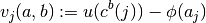
the vector of agents’ expected payoffs is defined by

$E(a,b,w):=((1-\delta)v_j(a,b)+\delta P^j(a_j)\cdot w)_{j\in \mathcal{Z}}.$

10.1. Outer Approximation: Conceptual¶

We can now define the outer approximation $\mathbf{B}^o(\mathcal{W})$ .

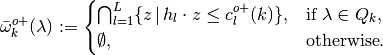
For each search subgradient $h_l\in H$ and each partition element $Q_k$ , let

(1) $c^{o+}_l(k):=\max_{(a,b) \in A \times B,\lambda\in Q_k, w}& [h_l \cdot E(a,b,w)], \\ \text{s.t.}\,\,&\lambda'=\lambda P(a), \\ & \lambda b^T \leq 0, \\ & w\in \tilde{\mathcal{W}}(\lambda', a), \\ & (1-\delta)\lambda \cdot v(a,b)+\delta \lambda' \cdot w\geq \check{\pi}_k,$
Then define

$\bar{\omega}^{o+}_k (\lambda) := \begin{cases} \bigcap_{l=1}^L \{z\,|\, h_l\cdot z\leq c^{o+}_l(k)\},& \text{if} \ \lambda \in Q_k,\\ \emptyset, & \text{otherwise}. \end{cases}$

Note

Since $A \times B$ is a finite set of action profiles, we can evaluate the program (1) as a special class of a nonlinear optimization problem–a nonseparable bilinear program (BLP)–for each fixed $(a,b) \in A \times B$ . Then we can maximize over the set $A \times B$ , by table look-up.

10.2. Outer Approximation: Implementation¶

Now we deal with implementing the idea in Outer Approximation: Conceptual. The outer-approximation scheme to construct $\mathbf{B}^o(\mathcal{W}^o)$ in the set of problems in (1) is computable by following the pseudocode below:

Pseudocode

Input: $H, c, \hat{\pi}, Poly$

For each $(Q_k,h_l,a) \in D \times H \times A$ :

Markov map $P \gets P(a)$

Simplex $T \gets P(Q_k)$

Get Hit-and-Run uniform draws constrained to be in $Q_k$ : $X:= \{ \lambda_n \}_{n=1}^{N_{sim}} \gets RandomPolyFill(N_{sim}, T)$

Get feasible set $F \gets F(B,Q_k) := \{ ( \lambda, b) \in Q_k \times B : \lambda \in X \subseteq Q_k, -\lambda b^T \geq \mathbf{0} \}$

Get $\mathbf{I}(a,k) := \{ k' \in \mathbf{K}: k' \mapsto Q_{k'} \in D, Q_{k'} \cap T \neq \emptyset$ }

Uses: TriIndex from Simplex_IntersectPmap

For each $k' \in \mathbf{I}(a,k)$ :

Get relevant feasible policy set $F(k'; a,k) \gets \{ (\lambda,b) \in F : \lambda P \in Q_{k'} \}$

For each $(\lambda,b) \in F(k';a,k)$ :

Get current payoff profile $v(a,b)$

Solve conditional LP:

$c_{+}^{o}(Q_k,h_l,a,k',\lambda,b) & = \max_{w} h_l [ (1-\delta)v(a,b) + \delta P w ] \\ s.t. & \\ H w & \leq c^{o}(Q_{k'}, h_l) \\ \delta[p^j(a')-p^j(a_j)]\cdot w & \leq (1-\delta) [\phi(a')-\phi(a_j)], \ \forall j \in \mathcal{Z} \\ -\lambda \delta P w & \leq \lambda [ (1-\delta)v(a,b) ] - \check{\pi}(Q_{k})$

Get $c_{+}^{o}(Q_k,h_l,a,k') = \max_{(\lambda,b) \in F(k';a,k)} c_{+}^{o}(Q_k,h_l,a, k',\lambda,b)$ .

Get $c_{+}^{o}(Q_k,h_l,a) = \max_{k' \in \mathbf{I}(a,k)} c_{+}^{o}(Q_k,h_l,a,k')$ .

Get $c_{+}^{o}(Q_k,h_l) = \max_{a \in A} c_{+}^{o}(Q_k,h_l,a)$ .

Note

In the pseudocode, we can see that for every fixed $(Q_k,a,k') \in D \times A \times \mathbf{I}(a,k)$ and every feasible $b$ , the nested family of programming problems are nonseparable bilinear programs (BLP) in the variables $(\lambda, w)$ .
The inner most loop thus implements our Monte Carlo approach to approximately solve for an $\epsilon$ -global solution to the nonseparable BLPs.
Conditional on each draw of $\lambda$ , this becomes a standard linear program (LP) in $w$ within each innermost loop of the pseudocode.
Given the set of subgradients $H$ , an outer-approximation update on the initial step correspondence $\mathcal{W}^o$ , is now sufficiently summarized by $\mathcal{W}^{o}_{+} = \mathbf{B}^o(\mathcal{W}^o) \gets (H,c_{+}^{o}(Q_k,h_l),\mathcal{W}^o)$ .

Relevant functions $\blacktriangleright$

Admit_Outer_LPset(self)¶

Returns:

Cnew :
- A $(L \times K)$ numeric array containing elements $c_{+}^{o}(Q_k,h_l)$ where $k \in \mathbf{K}$ and $h_l \in H$ are, respectively, a partition element of the correspondence domain $D$ , and, search subgradient in direction indexed by $l \in \{1,...,|H|\}$ .

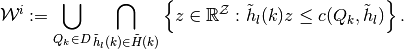
10.3. Inner Approximation: Conceptual¶

We now define the inner approximation of the SSE value correspondence operator as $\mathbf{B}^i(\mathcal{W})$ below.

Denote $\tilde{H}(k)$ as a finite set of $\tilde{L}(k)$ spherical codes (to be used as approximation subgradients, where each element is $\tilde{h}_l (k)$ and $\| \tilde{h}_l (k) \|_2 = 1$ for all $l = 1,...,\tilde{L}$ and $k \in \mathbf{K}$ .
Assume an initial inner step-correspondence approximation of some convex-valued and compact-graph correspondence

$\mathcal{W}^{i} := \bigcup_{Q_k \in D} \bigcap_{\tilde{h}_l (k) \in \tilde{H}(k)} \left\{ z \in \mathbb{R}^{\mathcal{Z}} : \tilde{h}_l (k) z \leq c(Q_k,\tilde{h}_l) \right\}.$

Define another finite set of fixed $L$ search subgradients, made up also of spherical codes, $H$ , just as in the outer approximation method above. [1]
For each search subgradient $h_l\in H$ and each partition element $Q_k$ , let

(2) $V^{i+}_l(k):=\min_{\lambda\in Q_k} \max_{(a,b) \in A \times B, w}& [h_l \cdot E(a,b,w)], \\ \text{s.t.}\,\,&\lambda'=\lambda P(a), \\ & \lambda b^T \leq 0, \\ & w\in \tilde{\mathcal{W}^i}(\lambda',a), \\ & (1-\delta)\lambda \cdot v(a,b)+\delta \lambda' \cdot w\geq \hat{\pi}_k,$

Set $V^{i+}_l(k) = -\infty$ if the optimizer set is empty.
In contrast to Outer Approximation: Conceptual, obtain the following additional step.
- Let $(a_{l}^{\ast}(k), b_{l}^{\ast}(k), w_{l}^{\ast}(k))$ denote the maximizers in direction $h_l$ and over domain partition element $Q_k$ , that induce the level $V^{i+}_l(k)$ above.
- Then the corresponding vector of agent payoffs is
$z^{+}_l (k) := E(a_{l}^{\ast}(k), b_{l}^{\ast}(k), w_{l}^{\ast}(k)).$
- Define the set of vertices 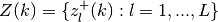$Z(k) = \{ z^{+}_l (k) : l = 1,...,L \}$ and let $\mathcal{W}^{i+}(k) = \text{co} (Z(k))$ .
Update

$Z^{+}(k) = \left\{ z^{+}_l (k) \in Z(k) : z^{+}_l (k) \in \partial\mathcal{W}^{i+}(k) \right\};$

and find approximation subgradients $\tilde{H}^{+}(k) = \{ \tilde{h}^{+}_1(k),...,\tilde{h}^{+}_{\tilde{L}^{+}}(k) \}$ and constants 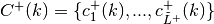$C^{+}(k) = \{c^{+}_1(k),...,c^{+}_{\tilde{L}^+}(k) \}$ such that

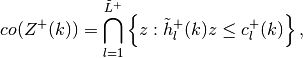
$co(Z^{+}(k)) = \bigcap_{l=1}^{\tilde{L}^{+}} \left\{ z: \tilde{h}_l^{+}(k) z \leq c^{+}_l (k) \right\},$

and $\mathcal{W}^{i+} = \cup_{k} co(Z^{+}(k)) = \mathbf{B}^i (\mathcal{W}^i)$ .

Note

As in the outer approximation methods, since $A \times B$ is a finite set of action profiles, we can evaluate the program (2) as a special class of a nonlinear optimization problem–a nonseparable bilinear program (BLP)–for each fixed $(a,b) \in A \times B$ . Then we can maximize over the set $A \times B$ , by table look-up. Thus, the only difference computationally in the inner approximation method is the extra step of summarizing each inner step-correspondence $\mathcal{W}^{i+}$ by updates on:

approximation subgradients in each $\tilde{H}^{+}(k)$ ;

levels in each $C^{+}(k)$ ; and

vertices, $Z^{+}(k)$ ,

for every $k \in \mathbf{K}$ .

Footnotes

[1]

Note that we have to let the approximation subgradients $\tilde{H}$ to possibly vary with domain partition elements $Q_k$ , as opposed to fixed search subgradients in $H$ used in the optimization step. This is because the former is endogenously determined by the extra convex hull operation taken to construct an inner step-correpondence $\mathcal{W}^{i}$ at each successive evaluation of the operator $\mathbf{B}^i$ .

Relevant functions $\blacktriangleright$

Admit_Inner_LPset(self)¶

Returns:

Znew :
- A $(L \times K)$ numeric array containing elements $z^{+}_l(k)$ where $k \in \mathbf{K}$ and $l \mapsto h_l \in H$ are, respectively, a partition element of the correspondence domain $D$ , and, approximation subgradient in direction indexed by $l \in \{1,...,L\}$ .

10. Computing approximate SSE payoffs¶

10.1. Outer Approximation: Conceptual¶

10.2. Outer Approximation: Implementation¶

10.3. Inner Approximation: Conceptual¶

Table Of Contents

Previous topic